Principles of probability in one posting

Probability as normalised proportionality

Probabilities are just weights.  Normalised to sum to unity.  No negative weights are possible.  Any time you can assign some number $P(i)$ to a set of $n$ objects/events/occurrences, finite or infinite, such that $\sum_{i=1}^n  P(i)=1$.  It is a world of weights with lower bound 0 and upper bond 1.  Mathematically those probabilities don't have to mean anything.  They don't have to correspond to real world probabilities.  They just need to be a collective set of non-negative numbers which sum to 1.  That's it.  If the set of numbers have that, it is a proper probability.  How best to formally define this?  Make the objects be sets.

Sets are a useful ontology for mathematically approaching normalised proportionality

First, set your universe.  This is the set of all possible elementary (i.e. disjoint) outcomes.  In any experiment, precisely one of these elementary outcomes will occur.  So the probability of an elementary outcome occurring, but where we don't care which, is 1.  We call the superset of all these disjoint elementary outcomes the sample space, often $S$.  If we want to refer to 'impossible' then this corresponds nicely to the probability of the empty set, $P(\{\})=0$, which gives us our floor.

Core axiom of probability - union/addition of disjoint events.

The engine which drives all of the basic theorems of elementary probability theory is in effect a definition of the word disjoint in the context of probability.  

$P(\bigcup_{j=1}^{\infty}A_j) = \sum_{j=1}^{\infty} P(A_j)$.  In other words, if you want to know the combined total probability of a union of disjoint events, go ahead and just sum their individual probabilities.  So, as you can see, if we define an experiment as just the sum total of elementary outcomes (disjoint), then naturally, this full sum will result in 1.  This is the probabilistic version of 'something is bound to happen'.

Already, with this core axiom, together with the floor and ceiling statements - the statements of proportionality, namely $P(\{\})=0$ and $P(S)=1$, we can derive/define the following.  In what follows, our main trick is to see if we can define arbitrary events in ways which are disjoint.  We need to get to that point so that we can be justified in triggering the core axiom.  So we smash, smash, smash sets until we have a collection of homogeneously disjoint sets.  This allows us free reign in applying the core axiom.

Let' see how the two set theory terms, complementarity, $A^c$ and proper subset $\subseteq$ ought to work in probability.

Complementary sets $A$ and $A^c$ are already disjoint, so immediately we know that we can treat $P(A \cup A^c) $ using the core axiom, plus by definition of complementarity, $P(A \cup A^c) =1$.   This gives us $P(A) + P(A^c) =1$ and so $P(A^c) = 1 - P(A)$.    This is often a great problem solving tool since we may find it easier to find the probability of an event's complement than directly of the event itself.  A classic example is the birthday problem.

Now let's work on an inequality. If $A \subseteq B$ then $P(A) \leq P(B)$.  This is our first non-trivial case of 'smash smash smash'.  $A$ is inside $B$, which suggests that we can smash $B$ as the union of $A$ and, ...., something else.  Something disjoint to $A$.  How about $A\cup (B \cap A^c)$.  Now, $P(B)$ becomes $P(A\cup (B \cap A^c))$, and by the power of our core axiom, this is equivalent to $P(A) + P(B \cap A^c)$.  Our floor axiom tells us that no probability can be less than 0, so $P(B \cap A^c) \geq 0)$ and hence $P(B) \geq P(A)$.  This little inequality points in the direction of measure theory.

Knowing how to rank the probabilities of any given set in the probability space is a useful thing to know, but having to power to do addition is even better.  How can we generalise the core axiom to cope with sets which are not guaranteed to be disjoint?  Think of your classic two-sets-with-partial-overlaps Venn diagram.  If we want a robust calculus of probability, we need to crack this too.

In general, we just need to be more careful not to over-count the shared areas.  Here it should be clear that there is a 'smash smash smash' decomposition of the areas in this diagram into pieces which are properly disjoint.  And indeed there is.  Skipping on the details, we arrive at $P(A\cup B) = P(A) + P(B) - P(A \cap B)$.  This two case example of making sure you count each disjoint area precisely once, by adjusting, generalises to: $P(\bigcup_{i=1}^{n} A_i) $ can be represented as $\sum_i P(A_i)  - \sum_{i<j} P(A_i \cap A_j) +  \sum_{i<j<k} P(A_i \cap A_j \cap A_k) - \ldots + (-1)^{n+1}  P(A_1 \cap \ldots  A_n) $.  Think of this as the mathematical equivalent of an election monitor who is trying to ensure that each voter only votes once.

So now we have the addition of any events $A_i$ in the probability space.  Sticking with the voting analogy, we will now drop down from a level of high generality, to one where all elementary outcomes are equally probable.  Imagine an ideal socialist, hyper-democratic world with proportional representation.  As we have seen, we already have the election monitor who endures the technical validity of summation.  But in this political environment, we want each elementary outcome (voter) to cast a vote which is precisely the same weight as all other voters.  We also measure utility in the ruthlessly rational-sounding utilitarian way - namely that we decide on our political actions by asking the people, and counting their votes equally.  In this less general world, simply counting the number of votes for any given event is all we need to do, since all votes are worth the same as each other.  Once we have the counts, we can stop, since we can now create count-based probability distributions.  Here we're in the world of fair dice, well shuffled playing cards, randomly selected samples.  And for those problems, combinatorics helps.

Let's assume there's an experiment with $n$ elementary outcomes and some event $A$ can happen in $p$ of those.  then $P(A)$ can be measured as $p/n$.  

Multiplication rule - chaining experiments

Imagine you could perform an experiment with $n$ outcomes as often as you like, with precisely the same set of outcomes each time.  That is, the second performance of the experiment has no 'memory' of the first result.  Technically this property is called a Markov property.  There would be $n$ outcomes on that second experiment.  In total there would be $n \times n$ outcomes in the meta-experiment which consisted in doing the first, then doing the second.  But your second experiment might be a totally different one, with $m$ outcomes.  Nonetheless there would be $n \times m$ possible outcomes now in the new meta-experiment.

Temporal fungibility

Note that, since multiplication  is commutative, it doesn't much matter if you do experiment '2' before experiment '1' - you still get $n \times m$ outcomes.  A similar effect occurs when you're adding probabilities - since addition is commutative.  This temporal fungibility helps later on with Bayes' theorem.

Four sampling rules follow from the multiplication rule:

1.  Sampling $k$ from $n$ with replacement, selection ordering matters:  $n^k$
2.  Sampling $k$ from $n$ without replacement, selection ordering matters:  $\frac{n!}{(n-k)!}$
3.  Sampling $k$ from $n$ with replacement, selection ordering doesn't matter:  $\binom{n+k-1}{k}$
4.  Sampling $k$ from $n$ without replacement, selection ordering doesn't matter:  $\binom{n}{k}$

Mirror rule for binomial coefficient.  Picking the rejects

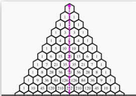When the team captain picks his preferred team, he's also implicitly picking his team of rejects.  Another way of saying this is that Pascal's triangle is symmetrical.  Another way of saying it is that $\binom{n}{k} = \binom{n}{n-k}$.  Again, this is a useful trick to remember in solving combinatoric problems.

L-rule for binomial coefficient

$\sum_{j=k}^n \binom{j}{k}=\binom{n+1}{k+1}$.  Or in pictures, all numbers like the number in yellow are the sum of the set of numbers in blue.  This collection of blue and yellow numbers is approximately like an L tilted.  This provides a useful decomposition or simplification, especially in cases where we have scenarios made up of a sum of binomial coefficients.  Cases like this and the below team captain decomposition relate a sum of binomials which in effect partitions the problem space in an interesting way, with a new binomial partition.  A partition generally is a complete and disjoint subsetting  of the problem space.  Here, we imagine one property in the population is rankable (eg age) with no ties.   So there is a population of $n+1$ in total and we picked this person to be in the selection group.  The partition is as follows:  imagine you pick your selection group; find the oldest in your group, and now start asking a series of questions about where this oldest in your group ranks in the overall population.  He could be the population oldest.  If so, then we define the rest of the group as $\binom{n}{k}$.  Perhaps he's the second oldest in the population.  If he's the second oldest in the population, then, by definition, we can't have picked the oldest from the population to be in our group (since we already found and identified our own oldest in group), so we know we must have $\binom{n-1}{k}$ other ways to satisfy this condition.  Continue along this path and you end up with the L rule.

The greatest.  Binary partitions for binomial coefficient

$\binom{n+1}{k} = \binom{n}{k} + \binom{n}{k-1}$.  The story here is : one of your population has a unique persistent property.  Now you come to chose $k$ from these $n+1$.  This is the same as the partition where your pick contains the prize winner and the other partition, where it doesn't.

Two tribes - Zhu Shijie (sometimes attributed to Vandermonde)

$\binom{m+n}{k} = \sum_{j=0}^k\binom{m}{j}  \binom{n}{k-j}$.  The story: Your entire population is made up of two tribes.  You have known sub-populations of each (ie you know the proportion).  You now pick your $k$.  This is the same as first segregating the populations into 2, then picking some number $j\leq k$ of the first tribe and, using multiplication rule on the second experiment, picking $k-j$ of the second tribe.  You run this for all possible values of $j$.

Lentilky. On tap at the factory, in dwindling supply in your pocket.

Forrest Mars, after telling his dad to "stick his Mars job up his ass" because he didn't get the recognition for the invention of the Milky Way, left for Britain in 1932.  By 1937, during the Spanish civil war, he was touring Spain with George Harris of Rowntree, they saw off-duty soldiers eating Lentilky, Moravian chocolate shaped like little lenses, covered with candy to stop the chocolate from melting. That idea was created by the Kneisl family, who had a factory in Holešov, making the stuff since 1907.  Harris and Mars decided to rip the idea off, and came to a gentleman's agreement to make Smarties in the UK and M&Ms in the USA.  Imagine a tube of Lentilky.  Each tube contains from 45 to 51 chocolate candies, of which there are 8 colours.  So how many possible tubes of Lentilky are there in total.  Ignoring for a moment the practical reality of the factory guaranteeing that you get probably roughly the same number of colours in each shape, let's allow all possibilities.

Step 1 in solving this is recognising it as a combinatorics problem.  Step 2 concentrates on one of the box cardinalities - say the tube with 45 sweets.  Step 3 recognise that this is sampling of $k$ from $n$, with replacement, order unimportant, $\binom{8+45-1}{8}$.  More generally, if the number of sweets is $i$, this is $\binom{8+i-1}{i}$.  That step is particularly non-intuitive, since $n$ is so much smaller a population than $k$, which you can only do in sampling with replacement.  Given they're unordered in the tube, order doesn't matter.  Step 4 applies the mirror rule, so that $\binom{8+i-1}{i} = \binom{i+7}{i} = \binom{i+7}{7}$.  Why do that step? Well, you've simplified the expression. But $i$ ranges from 45 to 51 of course, so there's a summation going on here: $\sum_{i=45}^{51}\binom{i+7}{7}$.  Step 5 simplifies the for range: $\sum_{j=52}^{58}\binom{j}{7}$; Step 6 rearranges to get $\sum_{j=7}^{58}\binom{j}{7} - \sum_{j=7}^{52}\binom{j}{7}$.  Step 7 is to use the L-rule, equating this to $\binom{59}{8} - \binom{53}{8}$.  My R session tells me the answer is 1,331,148,689 or about 1.3 billion.

Subset cardinality as binary encoding 
Consider a set with $n$ members - surely a candidate for one of the most generalised and useful objects in all of mathematics.  Free from any representation, not tied down to a semantics.  Just $n$ objects.  How many subsets of this general set are there?  Transform this question into the following recipe for enumerating all proper subsets.  Imagine a register with $n$ bits.  Each possible value of this register represents precisely one subset by virtue of the first bit being set representing the state that the first object is also in this subset, the second, third likewise.  The total number of values for an $n$ bit register is $2^n$, which is also therefore the cardinality of the number of subsets - including the null set and the original set itself.

Survival of the *est
Abstract example.  Take that set of $2^n$ subsets of the primordial set of $n$ objects.  Which of those has the largest cardinality?  Why the set containing all $n$ elements, of course.  Of course, only because we have this omniscient perspective on the set of all subsets of $n$.  But imagine we have a much more local  and limited capacity, namely that  we can select 2 of those $2^n$ subsets and face them off against each other.  The 'winner' is the largest (or the one which has the highest of any other rankable measure).  Imagine we do that for the whole set of randomly chosen ordered pairs.  We collect each winner and, just like a knockout tournament, we pair the winners off.  We repeat.  At the end, the last set standing is the largest, and it will of course be the set of all $n$ objects.  This knockout tournament is like a partially functional merge sort algorithm.  The full equivalence is when we let all the losers battle it out too.  But back to the tournament.  There are $\binom{n}{2}$ initial pairings, there are $n$ rounds in the competition and there are $2^n -1$ actual matches in the whole tournament.  The CPU of a computer is precisely such a localised, embodied, non-omniscient actor, and that actor needs an algorithm to achieve what a set-theory God can know merely by intuition.  The tournament or natural selection, or markets represent a local-space algorithm which results in a somewhat God-like perspective.

Sequential snap
Again assuming limits to knowledge, let's imagine all $n$ objects in our primordial set have permanently associated integers 1, 2 etc linked with them.  Now, again in a very non-set way, let's create a permutation of those $n$ objects.  With limited knowledge, we will model the probability that when we examine this permutation, object by object, that the object associated with the integer $i$ will be examined at the $i$th examination moment.  The likelihood that you win the game is independent of the value of $n$, rather surprisingly, at $1- \frac{1}{e}$

Probability preferences : the source of randomness is not the game

Fermat's version of the solution to the problem of points was to create a grid of possibilities reaching fully out to the point beyond which no doubt could exist as to who the winner would be.  This grid of possibilities included parts of the tree which, on one view, would be utterly irrelevant to the game in hand, and on another view, incorrectly modelled the set of possibilities embedded in the game.

Pascal's solution, by way of contrast, was a ragged tree of possibilities stretching out along each branch only as far as was needed to resolve the state of the game in question, and no further.

Pascal additionally made the mistake, in interpreting Fermat's solution, of ignoring order when tossing three dice/coins and in this mis-interpretation came up with an answer in the case of three players which diverged from his own reverse recursive solution based on the principle of fair treatment at each node of his ragged tree.

Because Pascal's wrong-headed idea of Fermat's solution did not match his own, he jumped to the conclusion that what must be wrong in Fermat's method was the extension of the tree of possibilities beyond those parts which the game in hand required.  Pascal consulted Roberval on the likely legitimacy of this fully rolled out tree of possibilities and Roberval seems to have told Pascal that this is where Fermat is going wrong, namely that this 'false assumption' of theoretical play of zombie-games leads to bad results.  It doesn't.

The evolution in time of a source of randomness was seen clearly by Fermat as separate from the rule, game or activity sitting on top of it.  In this case the game was the 'first to get N wins'   Modern derivatives when tree based methods are used all apply this same move.  First the random process's set of possibilities are evolved on a lower, supporting layer, then the payoff of the contract is worked out at the terminal time horizon.  Both in De Mere's game and with an option, there's a clearly defined termination point.  With De Mere's game, the point happens when the first player reaches N wins.  With options, the termination point is the expiry of the option.  Gambler's ruin, as I'll discuss later, doesn't have such a straightforward termination point.  So step 1 is to lay out all the possible states from now to the termination point, the tree of possibilities for the stochastic process.  Then you work out the terminal value of the contract or game and use Pascal's fairness criterion to crawl back up the second tree, until you reach the 'now' point, which gives you the fair value of the contract.  This is the essence of the finite difference solution set, and it works for path dependent and path independent pricings.  The implications of the game is that the tree is re-combinant, which means the binomial coefficients become relevant when working out the probability that each path is traversed.

Fermat has a clearer and earlier conception of this separation.  But Roberval and Pascal were right to flag this move up - what grounds did Fermat give for the move?  In modern parlance, we can see that the stochastic process, often a stock price or a spot FX or a tradeable rate, is independently observable in the market.  But back then, Pascal was struggling to separate the game from the source of randomness.  F. N. David suggests that Pascal sets Roberval up as the disbeliever as a distancing mechanism for his own failure to grasp this point.  Likewise, David suggests perhaps Pascal only solved his side of the problem after initial prompting from Fermat, in a letter which starts off the correspondence but which unfortunately no longer exists.

Of course, this isn't a solution of an unfinished game, but the fair value of the game at any point during its life. Each author I read seems clear in his mind that one other other of the great mathematicians' solution is preferred.  Is this just ignorance, aesthetic preference masquerading as informed opinion?  Yes, largely.  But my own opinion is that the both solutions share many similarities - both need to evolve a tree of possibilities, a binary tree, for which the binomial coefficients come in handy as the number of steps increases.  Both then involve evaluating the state of the game at the fixed and known horizon point.  Fermat's tree is a set of possibilities of a stochastic process.  His solution takes place exclusively at that final set of terminal nodes, but working out the ratio of the set of nodes in which player A is the winner over the total set of terminal nodes.  Pascal's tree is the tree of game states.  He reasons in a reverse iterative way until he reaches the start point, and the start point gives him his final answer.  The arithmetic triangle could help both these men build their trees as the number of steps increases.

Probability Preferences: Event Space is primary, Equi-probable Event Space is secondary

Technically, probabilities are proportions, fractions of a nominally unitary whole.  Those proportions don't have to be the same size.  When they are, then counting tricks, combinatorics, can come into play.  In my four walls metaphor for probability the first wall is made up of bricks of uneven areas.  This the primary case in probability theory.  Understanding that you have an event space and that you sum regions of a unitary whole, this is all that you need.  With equally-sized areas, number theory tricks become relevant, since there's a mapping from each area to a whole number, and you arrive at your proportion by scaling it down by the sum of all such elementary outcomes, $\sum_n 1$

It is hugely important in my mind to see where and when numbers come into it all and at what stage.  Unevenly sized elementary outcomes don't map neatly to the whole number system, and that's OK.  On a related point, the event in question, elementary or otherwise, doesn't have to have a mapping on to a number either.  If it does, then you further can talk about expectations, functions of random variables, etc.  But you don't need that either.  What distinguishes an equi-probable random device is that this probability distribution is the maximum entropy one (2.58 bits in the case of a die, 1 in the case of a coin).  The mimimal entropy case for all randomisation devices is the one where all elementary outcomes, regardless of how biassed or unbiased the device is, map to one event.  In that case the information content is 0 and technically it is no longer a randomisation device, you've effaced its randomness, so to speak.  What makes these proportions of a unitary whole interesting is that, for any given activity, game or contract with randomness, there's a particular configuration of thee probabilities in your mathematical analysis which come close to the results you would expect if you carried out the experiment multiple times.

Isaac Todhunter's "History of the mathematical theory of probability from the time of Pascal to that of Laplace", 1865, is a key milestone in the history of probability theory.  F.N. David, also often quoted by many of the authors I've read, references Todhunter thus: "[he].. has been and always will be the major work of reference in this subject" (F.N. David, preface, ix).  Ian Hacking, in his amazing "The emergence of probability" says in the first sentence of chapter 1 "[Todhunter]...remains an authoritative survey of nearly all work between 1654 and 1812" (Hacking, p1).  Todhunter's very book title is revealing - he originates probability theory with Pascal.  This choice echoes down through all the probability books I've come across.

Todhunter was a senior wrangler, so his intellectual capacity is beyond doubt (just check out the list of former senior wranglers and the equally stellar top 12's).  He describes Cardano's "On casting the die" as a 15 page gambler's manual where ".. the discussions relating to chances form but a small portion of the treatise" (Todhunter, p2).

Cardano discusses the activity of throwing two dice and summing the number of pips across the two dice.  He lays out the theory of probability as 'proportions of a unitary whole' using the language of 'chances'.  That he chose dice rather than astragali is of merely historical interest since no doubt he is the first in the western tradition to make this proportions-as-chances analogy.  Cardano also nails the implications of all 36 elementary outcomes on the activity of 'summing the pips', which involves understanding that rolling two dice implicitly maintains a knowledge of which die is which.  In a sense, that each die is 'result-reading colour coded'.  In  a previous book he also talks about binomial coefficients, for which Pascal usually gets credit.  He performs the same analysis for three dice.  As I'll mention in a subsequent post (on parallel/sequential irrelevance), this is theoretically equivalent to predicting the future three steps out.  Keith Devlin in "The unfinished game" explicitly (and wrongly) gives Pascal and Fermat credit for this.

My suspicion is that this senior Wrangler naturally preferred the great mathematicians Pascal and Fermat and that he recoiled in disgust at the unloveable life which Cardano seems to have lived.  

F.N. David upgrades Cardano to ".. a little more achievement that Todhunter allows him but .. not .. much more" (F.N. David, p59).  Hacking ends his chapter on Cardano with this: "Do we not find all the germs of a reflective study of chance in Cardano?Yes indeed" (Hacking, p56).

Did Cardano understand the primacy of the 'variable sized brick' case?  Yes.  Hacking quotes this translated section from Cardano: "I am as able to throw 1,3 or 5 as 2,4 or 6.  The wagers are therefore laid in accordance with this equality if the die is honest, and if not, they are made so much the larger or smaller in proportion to the departure from true equality" (Hacking, p54).   F.N. David is not so sure since Cardano incorrectly treats of astragali as if they were equi-probable, though he admits this may just be due to Cardano's lack of experience with astragali.  Anyway, if not, surely you're allowed to totally mis-characterise one specific randomisation machine and still be the father of modern probability theory.

Credit spread is probability through a sausage machine. Volatility is probability through a juicer

Just as statistics is really an elaborate form of a particular kind of probability activity over sufficiently large numbers, then so too am I beginning to see the volatility of equity derivatives and the credit spread of the fixed income world as two other distinct kinds of mathematical context within which you can find probability theory applied.  And of course, probability is useful to us insofar as it can place a number on something ultimately unknowable.  Albeit a known unknown ('risk' or measurable uncertainty, in the Knightian sense).  My main point here is that credit spread and volatility, the two great inputs into fixed income and volatility modelling, are brothers.