Putting all your eggs in the saftest basket known to man

In the end it is somewhat ironic that Markowitz starts off being concerned that real investors don't do what was logically implied by the Burr Williams approach, namely to put all their investment in a single maximal $E[r']$.  This leads to the efficient frontier set of portfolios.  Yet if he would have put the risk free asset in there, his efficient frontier collapses down to a single line, replicating the capital market line anyway.

Isn't it weird also that no-one is concerned that the efficient portfolio, on its way to being the CML, remains nonlinear until the final moment.  It also flattens out the curvature and hence the juice, the value, of the free lunch, namely diversification.  The minimum variance portfolio which contains treasury bills, plus all of the stocks in the stock market, is one where you have 100% of your assets in bills.

Automating the journey along the Capital Market Line

With the arrival of the ill-fitting Capital Market Line onto the efficient frontier, that eternal Achilles heel of portfolio selection, the moment when the analyst has to go back to the investor and asks them where they prefer to be on the efficient frontier reappears as a question of where the investor ought to be on the Capital Market Line.  Markowitz had always been comfortable, having been taught by the Bayesian Jimmy Savage, with considering the expected returns and covariances as a modellable step.  Soon to come was Fama, telling the world that, at least up to that point, the observed price history of the security was the best model of stock returns, which somewhat distracted the intellectual impetus from producing a proper Bayesian framework, as per Black and Litterman.

However, I think even the self-estimate on how risk adverse the investor was could perhaps have been re calibrated as a decision, not a preference.  Making it a decision allows the tools of decision theory to be making suggestions here.  Rather like the potential claimed benefits of traffic smoothing, low insurance, low accident rates, fewer cars in a world of driverless cars.

When an investor is asked for his preference I presume he in effect is really making some kind of unspoken decision either then, or at some point in the past.  And after all, how stable, how low a variance, is attached to the investor's risk appetite.  Using words like 'appetite' make it sound like Keynes's 'animal spirits' inside the hearts of those people who make business investment decisions.   If there's in principle the idea of varying appetites, which of course lies behind the final stage of classic Markowitzian portfolio selection, then how rational can that set of disparate appetites be?

Asking the question opens the Pandora's box.  That same box which remains closed in other realms of seeming human freedom - the law, consumption of goods.

Here's my initial stab at offering a model which demonstrates simultaneously multiple appetites but with retaining an element of rationality.  That's not to say that a behavioural scientist can't spot irrational decisions in practice.  Rather like CAPM, this attempt to remain rational might provide an interesting theoretical framework.

Aged 90, if we're lucky, on our death bed, we don't need to worry too much any more about our future investments.  Clearly, the older you are, the more you can afford to backslide down the CLM towards the $R_f$ point, ceteris paribus.  Conversely the more your expected lifetime consumption is ahead of you, the more you'd be tempted to inch up the CML.

Trying to take each element separately is difficult since there are clearly relationships between them.  Element two is wealth.  Clearly the average person becomes wealthier the older they get.  But, assuming a more or less stable spending pattern, it could be argued (billionaires aside) that as wealth increases, the investor relaxes back down the CML.

Both these first two elements are in a loose sense endogenous; the third element, such that it can be known, would be exogenous - if you have a model which tells you how likely it is that there's going to be a recession, then that could drive you up and down the CML.

Perhaps what's needed is an overrideable automation switch for where the investor resides on the CML right now.  That is, a personalisation process which guides the investor, which demonstrates to the investor how they deviate from the average CML lifetime journey.

Element four could be mark to market performance. Say the investor has a short term institutional hurdle to overcome, e.g. they would be happy making 10% each year.  I.e. that they're not just maximising lifetime expected wealth but  have equally important short term goals. Let's say we count a year as running from October to September and the investor achieved 10% by April one year.  Perhaps he'd be content to step away from the volatility from April to September one year.  By asking an investor what their risk appetite is, you're already asking them to accept a non market return, since only those investors who stick stubbornly to the tangency portfolio will see this.  Most investors will spend most of their investment life somewhere between $R_f$ and M, probably closer to M.  So they will have accepted a lower expected return anyway.  Some portfolio managers and hedge fund managers already run their businesses akin to this - they have perhaps loose monthly or quarterly targets and will step off the gas deliberately on occasion on good periods.  Converse they might increase leverage disastrously if they feel they're in catch up, a move often described as doubling down after the famous Martingale betting strategy. 

The argument against element three above is as follows: first, many hedge funds have tried to beat the market.  Not many consistently do, and even less so do it for macro economic reasons.  No such an exogenous model could be built.  To its advantage would be the fact that this model trades only in highly liquid assets (e.g. e-minis and treasury bills) so this would reduce transaction costs.  Secondly, transaction costs these days can be built in as a constraint to the portfolio optimisation step.  Another point in its favour is that the economic model can be made to generate actionable signals at a very coarse level.  A counter-cyclical model, which pushes you up the CML when a recession has occurred, would be a first step (running the risk of all such portfolio insurances of the past); a second step would be a model which slightly accelerates the back sliding only after the period of economic expansion is well beyond the normal range of duration for economic expansions.  This second step in effect relies on there being some form of stability to the shape and duration of the credit cycle.

Leaving the investor's risk preferences as an unopened black box seems to be missing a trick.

Sharpe Hacks the Efficient Frontier Diagram

Markowitz didn't add the capital market line to his famous efficient frontier diagram.  The idea of a capital market line dates back at least as far as Irving Fisher, and it seems that Tobin, in his 1958 "Liquidity Preference as Behavior toward Risk", in which he references the earlier work of Markowitz, and asks the question: why would a rational investor ever own his government's 0 yield obligations (cash, to you and I) versus that same government's non-0 yielding bonds (or bills).

He could have considered, and perhaps he did think this way, interest-bearing government obligations as just one more asset to drop into the portfolio.  But, according to the following informative blog post on the subject of Tobin's separation theorem, there's a better way of doing this.  Before going into it in detail, note that the theory is becoming more institutionalised here by treating risk free lending as a separate element to the portfolio selection problem.  In effect, we've added a rather arbitrary and uniquely characterised asset.  Not only that, I've always thought the capital market line is a weird graft for Lintner (1965) and Sharpe (1964) to add on to the efficient portfolio diagram.

The efficient portfolio diagram is a $(\sigma, r)$ space, it is true, but in Markowitz's formulation, each vector in this space is also a collection or zero or more different portfolio combinations.  Whereas, when you add the CML, whilst it is true that the proportion $p$ of cash and $1-p$ of the market portfolio is at each point on the line is at that higher level a unique portfolio in its own right, we are coming from a semantic interpretation of the efficient frontier where each distinct point contains a different portfolio of risky assets.  On the CML, every point has precisely the same market portfolio, more or less watered down by a mix of the risky market portfolio (in general, the tangency portfolio, before we get to the CAPM step).  

As a side note Markowitz has been noticeably critical of the CAPM assumption on limitless lending and borrowing at the risk free rate, and unbounded short assumptions.  In other words, he's likely to approve of the CML from $R_f$ up to the point it hits the market portfolio, at which point, like a ghost train shunted on to the more realistic track, he would probably proceed along the rest of the efficient frontier.

Clearly, the tangency portfolio has the highest sharpe ratio, in any line emanating from the risk free rate at the ordinate.  Sharpe and Lintner were to argue that point happens to be the market portfolio (on the assumption that all investors had the same $E[r]$ and $E[\sigma^2]$ expectations and all cared only for these two moments in making their investment decisions.

The addition in this way of the tangency line always felt as if it were a geometric hack around the then costly step of having to run a brand new portfolio optimisation with treasuries added as the $N+1$th asset.  Remember, at this point the CAPM hasn't been postulated and the tangency portfolio was not necessarily the market portfolio, so the tangency portfolio was still going to have to be optimised.  However, the CML from $R_f$ to $M$, as it approaches $M$ is actually above (and hence better than) the original efficient frontier.  And again, if one was happy with the assumption that one can borrow limitlessly, then all points to the right of $M$ would be objectively higher and hence more preferred than those on the original efficient frontier.

However, how would they look when you plot the CML plus original efficient frontier together with the new efficient frontier with treasuries as the $N+1$th asset?  Clearly that new frontier would be closer to the line, and flatter.    And Markowitz would then ask the investor to chose where they want to be on the new $N+1$ (nonlinear) efficient frontier.  Also, linear regression of stocks via a sensitivity of $\beta_i$ to the market would not be such a done deal.

A further problem I have with the CML is that treasuries, even bills, most surely do have variance, albeit very small, and only if the one-period analysis matches precisely the maturity of the bill will there be no variance.  Perhaps on an $N+1$th efficient frontier, the CML isn't the one with the highest $\frac{R_p - R_f}{\sigma}$.  I can well imagine that, leaving the original CML on the graph, as you chart the new Markowitz $N+1$ frontier, then there'd be points along that new frontier which have better risk-return profiles that those of the CML associated with an $N$ portfolio.

As a matter of academic fact, Sharpe actually attached the CML to the efficient frontier first in his 1963 paper "A Simplified Model for Portfolio Analysis", where he very much sees the regression step which ultimately later leads to his concept of beta and which makes attachment to economic equilibrium theory as an optimisation step to reduce the number of estimable parameters.  In the same vein, he sees the CML (the idea for which he doesn't credit Tobin/Fisher, whereas a year later in his classic CAPM paper, he does credit Tobin - who himself doesn't credit Fisher) as a speedup only.  He says:

There is some interest rate $r_i$ at which money can be lent with virtual assurance that both principal and interest will be returned; at the least, money can be buried in the ground ($r_i=0$).  Such an alternative could be included as one possible security ($A_i = 1+r_i, B_i=0, Q_i=0$) but this would necessitate some needless computation.  In order to minimise computing time, lending at some pure interest rate is taken into account explicitly in the diagnonal code.

Wow.  What a poor reason, in retrospect, for doing it this way.  By 1964 he found his economic justification, namely that it theoretically recapitulated a classical Fisherian capital market line. But in 1963 it was just a hack.  Even his choice of variable name $A_i$ for $E[r_i]$ and $Q_i$ for $\sigma_i$ showed where his head was at - namely he was an operations research guy at this point, working with Markowitz in an operations research private firm.

At the very least, it seems to me, there's no theoretically good reason why we can't just add a risk free asset into the mix and do away with the CML.  That way, we'd get a touch of variance in the asset, and a degree of purity back, Markowitzian framework purity.  CAPM certainly is needed to produce beta, the major factor, but that after all is a function of the security market line, a different line.

The meat of Markowitz 1952

In the end, what Markowitz 1952 does is twofold:

First, it introduces the problem of minimisation of variance subject to constraints in the application context of portfolios of return-bearing entities.  Once introduced, the case of a small number of entities is solved geometrically.   By 1959, the preferred solution to this was the simplex method.  By 1972 Black noted that all you need is two points on the efficient frontier to be able to extrapolate all points.  By 2019 you have a plethora of R (and other) libraries which can do this for you.

Second, a connection is established with the then current economic theory of rational utility.  Here he sketches the briefest of arguments for whether his maxim (expected mean maximisation with expected variance minimisation) is a decent model of investment behaviour.  He claims that his rule is more like investment behaviour than speculative behaviour.  However he makes a typo (one of several I spotted).  He claims that, for his maxim  $\frac {\partial U}{\partial E} > 0$ but also that $\frac {\partial U}{\partial E} < 0$ whereas that second one should read $\frac {\partial U}{\partial V} < 0$.  His claim that his approximation to the wealth utility function, having no third moment, distinguishes it from the propensity to gamble.  It was t be over a decade later before a proper mathematical analysis of how the E-V shaped up as a possible candidate investor utility function, and, if so, what an equilibrium world would look like if every investor operated under the same utility function.

Markowitz and expectation

One of Harry Markowitz's aha moments comes when he reads John Burr WIlliams, on equity prices being the present value of future dividends received.  Markowitz rightly tightened this definition up to foreground the fact that this model works with some future uncertainty, so the phrase 'present value of future dividends' ought to be 'expected present value of future dividends'.  We are dealing with a probability distribution here, together with some variance expressing our current uncertainty.  When variance here is a now-fact, representing our own measure of ignorance, that fits well with a Bayesian/Information Theoretic framework.  

I note that in 1952 the idea of future expected volatility was very dramatically under-developed.  It was still two decades away from the Black-Scholes paper and the trading of listed equity options on exchange.  The term implied volatility was not in common finance parlance.  

The other interpretation of variance in Markowitz's classic Portfolio Selection, 1952 is that it ought to be the expected future variability in the stock's (or portfolio's, or asset's, or factor's) return.  That is, the first of Markowitz's two stages in selecting a portfolio is making an estimate of the expected return and expected variance of the return stream.

He says:

The process of selecting a portfolio may be divided into two stages. The first stage starts with observation and experience and ends with beliefs about the future performances of available securities. The second stage starts with the relevant beliefs about future performances and ends with the choice of portfolio. 

 I'm mentioning this since I think Markowitz thought of minimum variance as a tool in the 'decision making with uncertainty' toolbox, namely that it in effect operationalises diversification, something he comes into the discussion wanting to foreground more than it had been foregrounded in the last.

What has happened largely since then is that maximum likelihood historical estimates of expected return and expected variance have taken precedence.  Of course, this is convenient, but it doesn't need to be so.  For example, imagine that a pair of companies have just entered into an M&A arrangement.  In this case, historical returns tell only a part of the story.

Also, if you believe Shiller 1981, the realised volatility of stock prices in general over the next time period will be much greater than the volatility on show for dividends and perhaps also not much like the realised volatility for the time period just past.

Taking a step back even further, we are assuming that the expected mean and variance of the relevant expected distribution is of the sort of shape which can appropriately be summarised by a unimodal distribution with finite variance, and that these first two moments give us a meaningful flavour of the distribution.  But again, just think of the expected distribution of an acquired company in an M&A deal half way through the deal.  This isn't likely to be normal-like for example, and may well be bimodal.

Markowitz 1952, what it does and does not do

Portfolio Selection, the original paper, introduces mean variance optimisation, it sets quantities as weights, it prioritises risk as variance, it operationally defines risk as variance as opposed to e.g. semi-variance, it gives geometric demonstrations for portfolios of up to four securities.  It comes from an intellectual statistical pedigree which is pro Bayesian (Savage).  It briefly connects E-V portfolios with Von Neumann Morgenstern utility functions.  It deals with expected returns, expected correlations.  It is neutral on management fees, transaction costs, if you would like it to be, since you can adjust your raw expected returns to factor in expected costs.

It doesn't give a mathematical proof in $n$ securities.  It doesn't generalise to dynamic expectations models $E[r_{i,t}]$ but assumes static probability distributions $E[r_i]$.  It doesn't introduce the tangent portfolio (a.k.a. the market portfolio).  It doesn't treat cash as a distinguished and separate asset class to be bolted on at the end of a 'risky assets only' E-V analysis.  It doesn't postulate what would happen if everyone performed mean-variance optimisation in the same way, i.e. it doesn't perform an equilibrium analysis.  It doesn't draw the risk-free to tangent 'capital allocation line' as a mechanism for leverage.  It doesn't assume unlimited borrowing.  It doesn't allow short positions.   It doesn't give techniques for solving the optimisation problem.  It doesn't talk about betas.  It doesn't prove which sets of utility functions in the Von Neumann-Morgenstern space are in fact economically believable and compatible with the E-V efficiency.  It doesn't just assume you look at history to derive returns and correlations and your're done.

Taking Sharpe and Markowitz as canonical, I notice that Shape seems less enamoured with Bayesian approaches (he critiques some Robo-advisors who modify their MPT approach with Black-Littterman Bayesian hooks.  For seemingly different reasons, they both end up not embracing the market portfolio/tangential portfolio idea; in Markowitz's case it is because he doesn't agree with the CAPM model assumptions which theoretically get you to the market portfolio in the first place, and with Sharpe, it is because he moved his focus from the domain he considers as having been converted already to pro-CAPM approaches, namely the professional investment community focused on accumulation of wealth, towards the individual circumstances surrounding retirees, in the decumulation stage.  However, I think, if you strip away why he's allowing more realism and individuality into the investment decisions of retirees, it boils down to Markowitz's point also.  Namely that realistic model assumptions kind of kill many flavours of pure CAPM.

Markowitz v shareholder value

Isn't it strange that Markowitz taught us that when it came to returns, maximising value is a stupid idea, whereas when it comes to evaluating the behaviour of managers in firms, maximising value stands still alone as a universal goal in US/UK models of capitalism.

Or, spelled out a little, companies are allowed to act as though they have permission exclusively to increase the share price (and hence increase the period return on the share price) as their operational definition of the goal of maximising shareholder value as opposed, for example, to maximising risk adjusted expected returns.

If risk adjusted returns are the goal for investors in portfolios of stocks, then why aren't they also the goal for owners of individual stocks.

Shiller advice to Oil heavy central banks

By the way, in the same video, did Robert Shiller really advise Norway and Mexico to take up massive short oil futures positions just to get them on to the efficient frontier?  He forgets to mention here that in doing so in such a size, you're bound to impact the underlying oil market, adversely, so that cost needs to be written against the benefit you'd have in moving closer to a more efficient national portfolio.  Another cost would be the cost of all those short futures would increase the basis between oil futures and oil itself.  You'd be paying that price on an ongoing basis as each future rolled.   Thirdly there's the mark to market issue.  Fourth there's the issue of which magnitude to short, the extracted oil only?  The total resource in the country?  Not at all quite as clear cut advice as he makes it sound here.

portfolios of asset types can contain hidden correlation

The risk of creating portfolios with asset classes is that there is hidden correlation.  For example, Shiller in this lecture, around the 55 minute mark in explaining the virtues of efficient portfolios, claims that having stocks, bonds and oil in your portfolio in some combination is a good thing, since it reduces correlation.

Well, to carry that point of efficient E-V further, you end up wanting to dis-articulate stocks into factors, since some stocks are more heavily oil sensitive than others, some stocks, with stable and predicable dividends, are more like bonds than others.  Just leaving the object set of the portfolio at assets leaves some hidden correlation off the table.  

In a sense, then, factor models are ways of taking x-rays of a security to see how correlated they are to fundamental economic elements (oil, carry, momentum, etc.)

In the limit, I think a good model needs also an element on the cyclicity of factors.  The most stable, that is, acyclic, factors are already found and have reasonable stories which persist through business cycles.  But this doesn't mean the rest of the factor zoo is for the dump.  If they can be attached to a meaningful theory of the business or credit cycle, then a factors carousel can be created.   Not all correlations are linear and constant.  Some can by cyclic, so perhaps linear regression isn't the ideal form for producing and measuring these correlations.

But getting a nowcast or forecast of economic conditions is not easy, nor do I think it properly interacts with factor models.

Portfolios of what?

Markowitz clearly had portfolios of stocks in mind.  It is also possible to see cash as another asset in the mix there, and government bonds.  But why not strategies or asset classes or even factors.  I really like the idea of strategies-and-factors.  To make this clear, imagine there was a well represented tradable ETF for each of the major strategies, being macro economic, convertible arbitrage, credit, volatility, distressed, m&a, and equity long short, commodities, carry trade.  Furthermore imagine that the equity long/short was itself a portfolio of factors, perhaps even itself an ETF.

A portfolio of factors from the factor zoo makes for an interesting though experiment.  I realise just how important it is to understand the correlation between factors.

Also, in the limit, imagine a long stock and a short call option on the same stock.  Can delta be recovered here using the linear programming (or quadratic programming) approach?  Unlikely.  But it highlights one of the main difficulties of the portfolio approach of Markowitz - just how accurate (and stable) can our a priori expected returns and expected covariances be?  

Imagine a system whose expected returns and expected covariances are radically random on a moment by moment basis.  The meaning and informational content of the resulting linearly deduced $x_i$s must be extremely low.  There has to be a temporal stability in there for the $x_i$s to be telling me something.  Another way of phrasing that temporal stability is: the past is (at least a little bit) like the expected future.  Or perhaps, to be more specific, imagine a maximum entropy process producing a high variance uniformly distributed set of returns; the E-V efficient portfolio isn't going to be doing much better than randomly chosen portfolios.

Also, surely there ought to be a pre-filtering step in here, regardless of whether the portfolio element is a security or a factor or an ETF representing a strategy, or perhaps even an explicit factor which is based not on and ETF but on the hard groundwork of approximating a strategy.  The pre filtering strategy would look to classify the zoo in terms of the relatedness of the strategies, on an ongoing basis, as a way of identifying, today, a candidate subset of portfolio candidates for the next period or set of periods.  Index trackers (and ETFs generally) already do this internally, but it ought to be a step in any portfolio analysis.  The key question you're answering here is: find me the cheapest and most minimal way of replicating the desired returns series such that it is within an acceptable tracking error.

Markowitz the practical

The expected trajectory of the Markowitz story is, Harry gets randomly pointed to work on portfolio selection by an anonymous broker who he met in his supervisor's waiting room.  A couple of years later, randomly, William Sharpe turns up and asks Markowitz what should he work on for his own thesis, and out of this CAPM is born.   Both Sharpe and Markowitz get Nobel prizes for this, but, fast forward to 2005 and Markowitz publishes a paper which in effect, blows up the pure CAPM, his own baby.  No doubt, CAPM has been blown up many many times in the intervening 40 years, nonetheless it is somewhat surprising to see a 40 years later article from the father of modern portfolio theory criticising CAPM so roundly.

The paper in question is "Market Efficiency: A Theoretical Distinction and So What?".  Such a dismissive sounding title.  Unusually so given the academic norms, even for a publication like the Financial Analysts Journal.  I'm reading it as an argument which placed mean-variance efficient portfolios above CAPM-compliant market portfolios, and the attack is on the principle of unlimited borrowing (and/or shorting).  He very much assigns this assumption to his Nobel peer, Sharpe ( Lintner probably should be in that list too but he died seven years earlier).

He makes this rather bold claim: 

Before the CAPM, conventional wisdom was that some investments were suitable for widows and orphans whereas others were suitable only for those prepared to take on “a businessman’s risk.” The CAPM convinced many that this conventional wisdom was wrong; the market portfolio is the proper mix among risky securities for everyone. The portfolios of the widow and businessman should differ only in the amount of cash or leverage used. As we will see, however, an analysis that takes into account limited borrowing capacity implies that the pre-CAPM conventional wisdom is probably correct.

This in effect completely blows a hole in the primary element of CAPM and CAPM-related models which privilege the market portfolio as most efficient of all, and most universal.

I think Markowitz wants more life to accrue to mean-variance optimisation, for there to be more and varied applications of it, using credible, practical, defensible assumptions, assumptions which in the limit are person-specific.  He makes similar points in his Nobel speech when he says:

Thus, we prefer an approximate method which is computationally feasible to a precise one which cannot be computed. I believe that this is the point at which Kenneth Arrow’s work on the economics of uncertainty diverges from mine. He sought a precise and general solution. I sought as good an approximation as could be implemented. I believe that both lines of inquiry are valuable.

So his claim is he likes practicality, both in models and in assumptions.  It was at RAND, after all, where Sharpe met him, and where he met mister simplex, George Dantzig.  Optimisation research will get you prizes in computer science, but of course not in economics.  It is worth mentioning that Markowitz also made strides in operations research (which I think of as a branch of computer science) - for example he was heavily involved in SIMSCRIPT and invented a related memory allocation algorithm for it, together with sparse matrix code.  The buddy allocation system made its way into linux, and hence in to pretty much every phone on the planet.  The very term sparse matrix was in fact coined by Markowitz.  So as you can see, his interests were very much algorithmic and practical, whether this was inside or outside of economics.

Markowitz the micro-economist of the investor

In 1990 Markowitz was awarded the Nobel prize, so I had a read of his short acceptance speech, which quite clearly sets the scene for his work.  He describes microeconomics as populated by three types of actor - the firm, the consumer and the investor (that last one being the actor he focuses on).  He then also interestingly creates binary divisions on work in on each of these three actors.  First, the individual and then the generalised aspect of their ideal behaviour.   How ought a firm best act?  A consumer?  An investor.  After having answered these questions, the generalisation is, how would the economy look if every firm, every consumer and every investor acted in the same way.

It is worth pausing on just this point about generalisation alone.  Clearly the question of uncertainty must raise its head to our modern ear.  Can one model all firms as following he same basic template, a so-called rational template?  If we can, then we may identify an economic equilibrium state.  Likewise, with consumers, how does an economy look if everybody is consuming according to the same basic utility function.  In both of these cases, whilst uncertainty is present, and known about by economic modellers, it is given a back seat.  Markowitz accepts this, but shows how it is literally impossible to background when it comes to the actions of the rational investor, since doing so leads to a model where every investor picks the single security with the largest expected return.  This does not happen, so any model which treats risk/uncertainty poorly is insufficient.

I think it is probably widely agreed that today, models of the firm's behaviour and of consumers' behaviour is best done with uncertainty built into the model.  The old linear optimisation models accepted that variability in firms, or consumers could be averaged away.  That is, that it was a valid approach to assume minimal uncertainty and see how, under those simplifying model assumptions, equilibrium models of the economy might be produced.

But fundamentally, portfolio investing in the absence of risk makes no sense at all.  In this case, in the limit, we find the portfolio with the best expected return, and put all our money in this.  However, not many people actually do that.  So, in the sense that the micro-economic models of the investor make claims to model actual behaviour, then uncertainty must play a more prominent role.

Markowitz also hands off on 'the equilibrium model of the investor' to Sharpe and Lintner's CAPM. He is happy to see basic portfolio theory as the element which attempts to model how people actually act (hence, a normative model) and leaves positive elements to Sharpe's theory, which I think he does so with only partial success.  But  certainly I see how he's keen to do so, especially since his mean variance functions are not in themselves utility functions, and in that sense don't touch base with economic theory as well as Arrow-Pratt.

Rather, looking back on his achievement, he makes a contrast between Arrow-Pratt and his own, perhaps more lowly contribution and praises his approach as computationally simpler.  This may be true, but it isn't a theoretically powerful defence.  However, I like Markowitz, I like his lineage, Hume, Jimmy Savage and the Bayesian statistical approach.  I'm happy to go along with his approach.

I notice how Markowitz gently chides John Burr Williams for describing the value of an equity as the present value of its future dividends, instead of describing it as the present value of its expected future dividends, that is to say, Markowitz draws out that these dividends ought to be modelled as a probability distribution, with a mean and with a variance.

Markowitz also highlights early on in his career that he reckons that downside semi-variance would be a better model of risk in the win-lose sense, but he notes that he's never seen any research which shows semi-variance captures a better model than variance.  This is a rather passive backing off of his original insight into semi-variance.  Did he not consider doing any real work on this?  Is it enough for him to note that he hasn't seen any papers on this?  However, it is certainly true that there isn't a huge numerical difference in equity index returns, usually, so I could well believe this doesn't matter as much as it sounds, though it would be good to know if someone has confirmed it isn't an important enough distinction.

What Markowitz in effect did was replace expected utility maximisation with an approximation function, which is a function of portfolio mean and portfolio variance, and then he, and others later, try to reverse this back in to particular shapes of utility function.  This is where the computer science algorithm of simplex, together with the ad hoc objective function involving maximising returns and minimising variance attempt to meet top quality economic theory, as expressed in Morgenstern and Von Neumann. 

Markowitz then spends the rest of his lecture showing how strongly correlated mean-variance optimisation is with believable utility functions.

He wraps up, as I'm sure many good Nobel laureates do, by talking about new lines of research.  Here, he lists three: applying mean variance analysis to data other than just returns.  He refers to these as state variables.  They too could have a mean-variance analysis applied to them.  Semi-variance, as mentioned already, is another possible new line of development, and finally he mulls over the seemingly arbitrary connection between certain utility functions and his beloved mean-variance approach.    The slightly point here is that all three of these potential lines of investigation were already candidates back in 1959, yet clearly here is Markowitz in 1990 repeating them as issues still.  

Where Portfolio Selection sits

Markowitz  (1952) is in effect a connection made between a piece of new computer science (linear programming and techniques such as simplex, and generally constrained optimisation solutions which arose out of the second world war) and an application in financial theory.  He tells the admirably random story of how he was waiting to see his professor when he struck up a conversation with another guy in the room, waiting to see the same professor, the guy being a broker, who suggested to Markowitz that he should apply his computer science algorithms skill to solving finance problems.

And given this random inspiration, he later finds himself in a library reading a book by John Burr Williams and he has a moment of revelation, namely that when you consider portfolios, the expected return on the portfolio is homogeneously just the weighted average of the expected returns of the component securities and so if this was the only criterion which mattered, your portfolio would just be 100% made up of that single portfolio which had the highest expected return.  You might call this the ancestral 'absolute alpha' strategy.  In knowing this single criterion was silly, he drew upon his liberal arts background, his knowledge of the Merchant of Venice, Act 1 Scene 1, as well as his understanding of game theory, particularly the idea of an iterated game and the principle of diversification, to seek out variance as an operational definition of risk.

He now had two dimensions to optimise, maximise returns whilst simultaneously minimise variance.  And finally, when he looks at how portfolio variance is calculated, he has his second moment of inspiration, since this is not just a naive sum of constituent variances, no, the portfolio variance calculation is a different beast.  This feeling, that the behaviour of the atoms are not of the same quality as the behaviour of the mass, is perhaps also what led John Maynard Keynes to posit a macro-economics which was different in quality to the micro- or classical economics of his education.

With normalised security quantities $x_i$ the portfolio variance is $\sum_i \sum_j x_i x_j \sigma_{i,j}$.

His third great moment was in realising that this was a soluble optimisation program, soluble in the case of two or three securities geometrically, but soluble in the general case with linear programming.  Linear programming also allowed for linear constraints to be added, indeed demanded that some be the case; for example that full investment occur, $\sum_i x_i = 1$, and that you can't short, $\forall i, x_i>0$.

However, notice the tension.  We humans often tend to favour one end of the normal distribution over another whereas mathematics doesn't care.  Take the distribution of returns, we cherish, desire even, the right hand side of the returns distribution and fear the left hand side.  So maximising the return on a portfolio makes good sense to us, but variance is not left or right handed.  Minimising variance is minimising the positive semi-variance and minimising the negative semi-variance too.  This is, so to speak, sub-optimal.  We want to avoid downside variance, but we probably feel a lot more positively disposed to upside variance.  Yet the mathematics of variance is side-neutral, yet we plug straight into that maths.

Gut, Optimisation, Gut

The way that Markowitz (1952) introduces mean variance optimisation to the financial world is as a maths sandwich between two slices of guts.  I think in the end, both those pieces of gut will prove amenable to maths too.  The first piece of so called guts is Markowitz's 'step one', the idea that one arrives though experience and observation at a set of beliefs (probabilities) concerning future expected performances (general term there, think returns, risks) on a set of risky securities.

For me, this sounds like it was already anticipating Black Litterman, 1990 approach, which was in effect to operationalise experience and observation in a process of Bayesian probabilistic modelling.  This approach is itself a form of constrained optimisation, rather like the techniques in linear programming, for example with Lagrange multipliers.  The Bayesian approach is of course not limited to linear assumptions.

Prior to 1952,  Kantorovich and then Dantzig has produced solutions to linear programming problems.  Dantzig, for example, had invented the simplex method when he misinterpreted his professor Jerzy Neyman's list of unsolved problems as a homework exercise, and went ahead and solved it.  

So Markowitz goes into this paper knowing there's a solution to his 'step 2', being an optimisation of both mean and variance in a portfolio.

Finally, the second slice of gut involves investors deciding which level of return they want, given their preference for the level of risk they're prepared to bear.  I think too, in time, this will be amenable to a mathematical solution.  That is to say, their level of risk can, to take only a single example, can become a function of a macro-economic model.

Covariance

If  $X$ and $Y$ are random variables then their covariance is the expected value of the product of their deviations from their means.  Or in mathematical form, $\sigma_{X,Y}=E[(X-E[X]) (Y-E[Y])]$.  There's a lot of juice in this idea, a lot. But interpreting it can be hard, since the value's meaning depends heavily on the units of $X$ and $Y$.  For example of $X$ and $Y$ are return streams, if you represent the returns as percentages, e.g. 4%, 3.5%, etc versus representing them as unit fractions, e.g. 0.04, 0.035, etc, then the covariance of one would be 10,000 times larger than the covariance of the other.

You can see that the variance is in fact just the self-covariance.  That is $\sigma_X^2 = \sigma_{XX} = E[{(X-E[X])}^2]$.  So going back to the covariance between two random variables, the largest possible value for the covariance of $X$ and $Y$ is going to be when $Y$ moves exactly like $X$, is in fact $X$.  

A useful way to normalise covariance was presented by Auguste Bravais, an idea which Pearson championed.  In it, the units of covariance are normalised away by  the product of the standard deviations of the variables.  The resulting measure, normalised covariance, which ranges from -1 to +1 had become better known as the Pearson correlation coefficient, or simply the correlation, or COVAR() in excel.  $\rho_{X,Y} = \frac{\sigma_{X,Y}}{\sigma_X \sigma_Y}$.  This is easier for humans to read, comprehend and for various covariances from different contexts to be compared and ranked.  But if you are building a square variance-covariance matrix, you now know it is just a covariance matrix.  Furthermore, if you square this normalised covariance, you arrive at the familiar $R^2$ measure, the coefficient of determination, which is also equal to the proportion of the variance explained by the model, as a fraction of the total dependent variable variance, being $\frac{\sigma_{\hat{Y}}^2}{\sigma_{Y}^2}$.

If $X$ is the return stream of an equity, and $Y$ is the return of the market, then by dividing the covariance by the variance of the market return, $\sigma_Y^2$, we end up with the familiar beta of the stock, $\beta_X = \frac{\sigma_{X,Y}}{\sigma_Y^2}$.  Notice how similar this is to the so-called Pearson correlation coefficient.  In fact $\beta_X = \rho_{X,Y} \times \frac{\sigma_X}{\sigma_Y}$.  That is to say, when you scale the correlation of the security returns to the market by a scaling factor of the security returns volatility per unit of market returns volatility, you get the beta.  Beta as correlation times volatility ratio, that makes sense for a beta.

Finally, 3 rules: 

1. if $Y =V+W$ then $\sigma_{X,Y} = \sigma_{X,V} + \sigma_{X,W}$
2. if $Y =b$ then $\sigma_{X,Y} =0$
3. if $Y=bZ$ then $\sigma_{X,Y} = b \times \sigma_{X,Z}$ 

And of course it is on the basis of rule (1) that Sharpe makes the development from Markowitz.

Principles of probability in one posting

Probability as normalised proportionality

Probabilities are just weights.  Normalised to sum to unity.  No negative weights are possible.  Any time you can assign some number $P(i)$ to a set of $n$ objects/events/occurrences, finite or infinite, such that $\sum_{i=1}^n  P(i)=1$.  It is a world of weights with lower bound 0 and upper bond 1.  Mathematically those probabilities don't have to mean anything.  They don't have to correspond to real world probabilities.  They just need to be a collective set of non-negative numbers which sum to 1.  That's it.  If the set of numbers have that, it is a proper probability.  How best to formally define this?  Make the objects be sets.

Sets are a useful ontology for mathematically approaching normalised proportionality

First, set your universe.  This is the set of all possible elementary (i.e. disjoint) outcomes.  In any experiment, precisely one of these elementary outcomes will occur.  So the probability of an elementary outcome occurring, but where we don't care which, is 1.  We call the superset of all these disjoint elementary outcomes the sample space, often $S$.  If we want to refer to 'impossible' then this corresponds nicely to the probability of the empty set, $P(\{\})=0$, which gives us our floor.

Core axiom of probability - union/addition of disjoint events.

The engine which drives all of the basic theorems of elementary probability theory is in effect a definition of the word disjoint in the context of probability.  

$P(\bigcup_{j=1}^{\infty}A_j) = \sum_{j=1}^{\infty} P(A_j)$.  In other words, if you want to know the combined total probability of a union of disjoint events, go ahead and just sum their individual probabilities.  So, as you can see, if we define an experiment as just the sum total of elementary outcomes (disjoint), then naturally, this full sum will result in 1.  This is the probabilistic version of 'something is bound to happen'.

Already, with this core axiom, together with the floor and ceiling statements - the statements of proportionality, namely $P(\{\})=0$ and $P(S)=1$, we can derive/define the following.  In what follows, our main trick is to see if we can define arbitrary events in ways which are disjoint.  We need to get to that point so that we can be justified in triggering the core axiom.  So we smash, smash, smash sets until we have a collection of homogeneously disjoint sets.  This allows us free reign in applying the core axiom.

Let' see how the two set theory terms, complementarity, $A^c$ and proper subset $\subseteq$ ought to work in probability.

Complementary sets $A$ and $A^c$ are already disjoint, so immediately we know that we can treat $P(A \cup A^c) $ using the core axiom, plus by definition of complementarity, $P(A \cup A^c) =1$.   This gives us $P(A) + P(A^c) =1$ and so $P(A^c) = 1 - P(A)$.    This is often a great problem solving tool since we may find it easier to find the probability of an event's complement than directly of the event itself.  A classic example is the birthday problem.

Now let's work on an inequality. If $A \subseteq B$ then $P(A) \leq P(B)$.  This is our first non-trivial case of 'smash smash smash'.  $A$ is inside $B$, which suggests that we can smash $B$ as the union of $A$ and, ...., something else.  Something disjoint to $A$.  How about $A\cup (B \cap A^c)$.  Now, $P(B)$ becomes $P(A\cup (B \cap A^c))$, and by the power of our core axiom, this is equivalent to $P(A) + P(B \cap A^c)$.  Our floor axiom tells us that no probability can be less than 0, so $P(B \cap A^c) \geq 0)$ and hence $P(B) \geq P(A)$.  This little inequality points in the direction of measure theory.

Knowing how to rank the probabilities of any given set in the probability space is a useful thing to know, but having to power to do addition is even better.  How can we generalise the core axiom to cope with sets which are not guaranteed to be disjoint?  Think of your classic two-sets-with-partial-overlaps Venn diagram.  If we want a robust calculus of probability, we need to crack this too.

In general, we just need to be more careful not to over-count the shared areas.  Here it should be clear that there is a 'smash smash smash' decomposition of the areas in this diagram into pieces which are properly disjoint.  And indeed there is.  Skipping on the details, we arrive at $P(A\cup B) = P(A) + P(B) - P(A \cap B)$.  This two case example of making sure you count each disjoint area precisely once, by adjusting, generalises to: $P(\bigcup_{i=1}^{n} A_i) $ can be represented as $\sum_i P(A_i)  - \sum_{i<j} P(A_i \cap A_j) +  \sum_{i<j<k} P(A_i \cap A_j \cap A_k) - \ldots + (-1)^{n+1}  P(A_1 \cap \ldots  A_n) $.  Think of this as the mathematical equivalent of an election monitor who is trying to ensure that each voter only votes once.

So now we have the addition of any events $A_i$ in the probability space.  Sticking with the voting analogy, we will now drop down from a level of high generality, to one where all elementary outcomes are equally probable.  Imagine an ideal socialist, hyper-democratic world with proportional representation.  As we have seen, we already have the election monitor who endures the technical validity of summation.  But in this political environment, we want each elementary outcome (voter) to cast a vote which is precisely the same weight as all other voters.  We also measure utility in the ruthlessly rational-sounding utilitarian way - namely that we decide on our political actions by asking the people, and counting their votes equally.  In this less general world, simply counting the number of votes for any given event is all we need to do, since all votes are worth the same as each other.  Once we have the counts, we can stop, since we can now create count-based probability distributions.  Here we're in the world of fair dice, well shuffled playing cards, randomly selected samples.  And for those problems, combinatorics helps.

Let's assume there's an experiment with $n$ elementary outcomes and some event $A$ can happen in $p$ of those.  then $P(A)$ can be measured as $p/n$.  

Multiplication rule - chaining experiments

Imagine you could perform an experiment with $n$ outcomes as often as you like, with precisely the same set of outcomes each time.  That is, the second performance of the experiment has no 'memory' of the first result.  Technically this property is called a Markov property.  There would be $n$ outcomes on that second experiment.  In total there would be $n \times n$ outcomes in the meta-experiment which consisted in doing the first, then doing the second.  But your second experiment might be a totally different one, with $m$ outcomes.  Nonetheless there would be $n \times m$ possible outcomes now in the new meta-experiment.

Temporal fungibility

Note that, since multiplication  is commutative, it doesn't much matter if you do experiment '2' before experiment '1' - you still get $n \times m$ outcomes.  A similar effect occurs when you're adding probabilities - since addition is commutative.  This temporal fungibility helps later on with Bayes' theorem.

Four sampling rules follow from the multiplication rule:

1.  Sampling $k$ from $n$ with replacement, selection ordering matters:  $n^k$
2.  Sampling $k$ from $n$ without replacement, selection ordering matters:  $\frac{n!}{(n-k)!}$
3.  Sampling $k$ from $n$ with replacement, selection ordering doesn't matter:  $\binom{n+k-1}{k}$
4.  Sampling $k$ from $n$ without replacement, selection ordering doesn't matter:  $\binom{n}{k}$

Mirror rule for binomial coefficient.  Picking the rejects

When the team captain picks his preferred team, he's also implicitly picking his team of rejects.  Another way of saying this is that Pascal's triangle is symmetrical.  Another way of saying it is that $\binom{n}{k} = \binom{n}{n-k}$.  Again, this is a useful trick to remember in solving combinatoric problems.

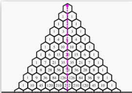
L-rule for binomial coefficient

$\sum_{j=k}^n \binom{j}{k}=\binom{n+1}{k+1}$.  Or in pictures, all numbers like the number in yellow are the sum of the set of numbers in blue.  This collection of blue and yellow numbers is approximately like an L tilted.  This provides a useful decomposition or simplification, especially in cases where we have scenarios made up of a sum of binomial coefficients.  Cases like this and the below team captain decomposition relate a sum of binomials which in effect partitions the problem space in an interesting way, with a new binomial partition.  A partition generally is a complete and disjoint subsetting  of the problem space.  Here, we imagine one property in the population is rankable (eg age) with no ties.   So there is a population of $n+1$ in total and we picked this person to be in the selection group.  The partition is as follows:  imagine you pick your selection group; find the oldest in your group, and now start asking a series of questions about where this oldest in your group ranks in the overall population.  He could be the population oldest.  If so, then we define the rest of the group as $\binom{n}{k}$.  Perhaps he's the second oldest in the population.  If he's the second oldest in the population, then, by definition, we can't have picked the oldest from the population to be in our group (since we already found and identified our own oldest in group), so we know we must have $\binom{n-1}{k}$ other ways to satisfy this condition.  Continue along this path and you end up with the L rule.

The greatest.  Binary partitions for binomial coefficient

$\binom{n+1}{k} = \binom{n}{k} + \binom{n}{k-1}$.  The story here is : one of your population has a unique persistent property.  Now you come to chose $k$ from these $n+1$.  This is the same as the partition where your pick contains the prize winner and the other partition, where it doesn't.

Two tribes - Zhu Shijie (sometimes attributed to Vandermonde)

$\binom{m+n}{k} = \sum_{j=0}^k\binom{m}{j}  \binom{n}{k-j}$.  The story: Your entire population is made up of two tribes.  You have known sub-populations of each (ie you know the proportion).  You now pick your $k$.  This is the same as first segregating the populations into 2, then picking some number $j\leq k$ of the first tribe and, using multiplication rule on the second experiment, picking $k-j$ of the second tribe.  You run this for all possible values of $j$.

Lentilky. On tap at the factory, in dwindling supply in your pocket.

Forrest Mars, after telling his dad to "stick his Mars job up his ass" because he didn't get the recognition for the invention of the Milky Way, left for Britain in 1932.  By 1937, during the Spanish civil war, he was touring Spain with George Harris of Rowntree, they saw off-duty soldiers eating Lentilky, Moravian chocolate shaped like little lenses, covered with candy to stop the chocolate from melting. That idea was created by the Kneisl family, who had a factory in Holešov, making the stuff since 1907.  Harris and Mars decided to rip the idea off, and came to a gentleman's agreement to make Smarties in the UK and M&Ms in the USA.  Imagine a tube of Lentilky.  Each tube contains from 45 to 51 chocolate candies, of which there are 8 colours.  So how many possible tubes of Lentilky are there in total.  Ignoring for a moment the practical reality of the factory guaranteeing that you get probably roughly the same number of colours in each shape, let's allow all possibilities.

Step 1 in solving this is recognising it as a combinatorics problem.  Step 2 concentrates on one of the box cardinalities - say the tube with 45 sweets.  Step 3 recognise that this is sampling of $k$ from $n$, with replacement, order unimportant, $\binom{8+45-1}{8}$.  More generally, if the number of sweets is $i$, this is $\binom{8+i-1}{i}$.  That step is particularly non-intuitive, since $n$ is so much smaller a population than $k$, which you can only do in sampling with replacement.  Given they're unordered in the tube, order doesn't matter.  Step 4 applies the mirror rule, so that $\binom{8+i-1}{i} = \binom{i+7}{i} = \binom{i+7}{7}$.  Why do that step? Well, you've simplified the expression. But $i$ ranges from 45 to 51 of course, so there's a summation going on here: $\sum_{i=45}^{51}\binom{i+7}{7}$.  Step 5 simplifies the for range: $\sum_{j=52}^{58}\binom{j}{7}$; Step 6 rearranges to get $\sum_{j=7}^{58}\binom{j}{7} - \sum_{j=7}^{52}\binom{j}{7}$.  Step 7 is to use the L-rule, equating this to $\binom{59}{8} - \binom{53}{8}$.  My R session tells me the answer is 1,331,148,689 or about 1.3 billion.

Subset cardinality as binary encoding 
Consider a set with $n$ members - surely a candidate for one of the most generalised and useful objects in all of mathematics.  Free from any representation, not tied down to a semantics.  Just $n$ objects.  How many subsets of this general set are there?  Transform this question into the following recipe for enumerating all proper subsets.  Imagine a register with $n$ bits.  Each possible value of this register represents precisely one subset by virtue of the first bit being set representing the state that the first object is also in this subset, the second, third likewise.  The total number of values for an $n$ bit register is $2^n$, which is also therefore the cardinality of the number of subsets - including the null set and the original set itself.

Survival of the *est
Abstract example.  Take that set of $2^n$ subsets of the primordial set of $n$ objects.  Which of those has the largest cardinality?  Why the set containing all $n$ elements, of course.  Of course, only because we have this omniscient perspective on the set of all subsets of $n$.  But imagine we have a much more local  and limited capacity, namely that  we can select 2 of those $2^n$ subsets and face them off against each other.  The 'winner' is the largest (or the one which has the highest of any other rankable measure).  Imagine we do that for the whole set of randomly chosen ordered pairs.  We collect each winner and, just like a knockout tournament, we pair the winners off.  We repeat.  At the end, the last set standing is the largest, and it will of course be the set of all $n$ objects.  This knockout tournament is like a partially functional merge sort algorithm.  The full equivalence is when we let all the losers battle it out too.  But back to the tournament.  There are $\binom{n}{2}$ initial pairings, there are $n$ rounds in the competition and there are $2^n -1$ actual matches in the whole tournament.  The CPU of a computer is precisely such a localised, embodied, non-omniscient actor, and that actor needs an algorithm to achieve what a set-theory God can know merely by intuition.  The tournament or natural selection, or markets represent a local-space algorithm which results in a somewhat God-like perspective.

Sequential snap
Again assuming limits to knowledge, let's imagine all $n$ objects in our primordial set have permanently associated integers 1, 2 etc linked with them.  Now, again in a very non-set way, let's create a permutation of those $n$ objects.  With limited knowledge, we will model the probability that when we examine this permutation, object by object, that the object associated with the integer $i$ will be examined at the $i$th examination moment.  The likelihood that you win the game is independent of the value of $n$, rather surprisingly, at $1- \frac{1}{e}$

Combinatorics with Blitzstein and Hwang

Also from Blitzstein and Hwang, seven chess matches are played between players A and B.  How many ways can the final result be 4-3 to A?

In doing this question, I am reminded about how almost all of the difficult work in maths questions comes in unpacking the question.  This unpacking is also the act of modelling.  And it isn't easy when you're doing it from scratch.

So my initial thinking was to transform the problem into a counting problem.  We don't need to model B at all here - it can all be done in modelling how A gets those 4 points.  This is because each game has precisely one point to distribute, and that will certainly happen at the end of each game.  So B disappears from the analysis.  This is like the 'degrees of freedom' idea in statistics 

With only seven games, there's no way A could have finished with 4 points without at least one clear victory.  At the other end of chess playing competence is the possibility that A won 4 (and therefore lost 3).  Note also that the number of draws must always be 0 or some multiple of 2.

Now that B has been dispatched, we look at the triplet which is a result.  In general, there are the following four ways that 4-3 can result, were W=A win, D=draw, L=A loss:

• 1W 6D 0L
• 2W 4D 1L
• 3W 2D 2L
• 4W 0D 3L

Now we can use the 'degrees of freedom' trick one more time.  If you know two elements of this triplet, then you'll know for sure what the third element is.  So we don't need to model three distinct values for D,W and L. We only need two, but which two?

I always prefer to go for smaller numbers, and on that basis, I'd go for W + L.  We shall henceforth model only A's wins and losses, since A's draws are implied.

Now we have a sum of 4 possibilities.  Let's take them one by one. ${7} \choose {1}$  represents all 7 locations where that one win would happen.  We don't have losses since by implication all the six other slots were draws.  So for this sub-case, we're done.  Once we place the  win, we have no more variations to deal with.

  ${{7} \choose {2}} { {5} \choose {1}}$ represents first how we can distribute two wins among the seven games, then when that's done we have 5 unfilled slots which we need to drop one loss into.  We multiply those two together (choices multiply).

Similarly,   ${{7} \choose {3}} { {4} \choose {2}}$ represents 3W + 2L.  And finally   ${{7} \choose {4}} { {3} \choose {3}}$ represents the case where we drop in four wins, then all remaining slots contain the full set of 3 losses.

The final answer to the question is: ${{7} \choose {1}} + {{7} \choose {2}} { {5} \choose {1}}  + {{7} \choose {3}} { {4} \choose {2}} + {{7} \choose {4}} { {3} \choose {3}}$

R thinks this amounts to 357 different possible ways to arrive at a 4-3 result for A.

MISSISSIPPI scramble

How many ways are there, Blitzstein and Hwang ask, to permute the word Mississippi?  There are two approaches.  Broadly, we're in the 'naive probability' world where all possibilities are equally likely, so counting methods are going to be useful.

First, and this is generally a good strategy, we give all 11 letters a unique identity.  That is to say, the first s must be thought of as distinct to the second, third and fourth, and so on.  This is analogous to understanding that when you throw a pair of dice, logically there's always a first and second identity for each die. 

There are $11!$ ways (39,916,800) to permute the 11 'distinct' letters (multiplication rule, based on sampling without replacement).  That's more ways than there are actual people currently residing in Mississippi:

Looks like it would take another 500 years, at the current rate of population growth, before we'd run out of basic ways of sharing all the permutations of Mississippi with its inhabitants.

But at this point we want to throw away (divide out) certain permutations.  From a schoolteacher point of view, wherever those four s's landed up, we don't care about their particular order now.  In other words, we're making the conscious decision to consider an s like any other s.  And an i like any other i.  And a p like any other p.  A kind of homogenisation.  The m stands unique and proud at the head of the word.  But in terms of permutations, the m is the unmodelled case, since, when you've decided how to fill the 10 other slots using all your s's, i's and p's, then the m just has to go where it is told.  What a come down - tables turned on the m.

There are four s's, and four i's.  And we need to know how much not to care about their order.  If we did care for their order, then we could permute them $4!$ ways.  Similarly there are $2!$ orderings of p.  So we want to throw away in total  $4!4!2!$ of the $11!$, meaning that the 'schoolteacher's answer' (were all letters are considered homogeneous) is $\frac{11!}{4!4!2!}$.

The second solution is to break it down into 3 sections, each with a binomial 'n chose k' element.

Let's start with the s.  We have 11 slots and 4 of them.  So $11 \choose 4$.  Using the multiplication rule, you then could drop your 4 i's into any of the remaining 7 slots, $7 \choose 4$ and finally our two p's can take up any of the three remaining slots, $3 \choose 2$.  Again, m is the unmodelled, bossed about letter who must take the last slot, wherever that is.  

So,  it must be the case that $11!/4!4!2! = {11 \choose 4}{7 \choose 4}{3 \choose 2}$.

What does R have to say about that?

It agrees, and gives us the final (schoolteacher's) answer, 34,650 versus the 'radical identity' answer of 39,916,800.

So perhaps we could give the school teacher permutations just to the Hispanic residents (excluding Puerto Ricans, sorry).