Volatility is not uncertainty.

Twelve months ago a hedge fund was created.  Eleven months ago it made a 1% first month return; for -2% for its second month, and so on.  By now, its 12 monthly percent returns look like this: $\left\{1,-2,2,\frac{1}{2},\frac{3}{4},-\frac{1}{2},0,0,0,1,-3,-4\right\}$.  It is useful to distinguish where the uncertainty lies.

The sequence of returns are certain enough.  They're a part of history.  You can calculate their sample variance as $\sigma^2  = \frac{1}{11} \sum_{m=1}^{12}(r_i - \bar{r})^2$ where $\bar{r}$ is the average, $-0.27$ in this case.  And the sample historical volatility $\sigma = 1.8$.  These are all certain.  The calculated volatility tells you with certainty just how variable those returns were.

If I got the measurements of the sizes of the planets in our solar system, I could likewise calculate the population variance and volatility.  With certainty.  I'm not saying anything whatsoever about their likelihood of change in the future.

In the world of finance and investing, we usually perform two extra operations which introduce uncertainty.  First, we decide we want to consider the unknown future and rope in history to help us.  Second, we construct a reference model, random in nature, which we hypothesise has been generating the returns we have seen so far and which will continue to generate the returns likewise into the unknown future.  That's a big second step.

Without wanting right now to go into issues about how valid this is, or even what form the model might take, I'll jump right in and suggest that next month's returns are expected to come in between  $-2$% and $1.4$%.  As soon as we decided to make a prediction about the unknown future, we added a whole bunch of uncertainty.  By picking our model (which, after all, might be an inappropriate choice), we've added model uncertainty.  By assuming that the future is going to be like the past, we've expressed a level of trust in reality which emboldens us to apply volatility to reduce all the uncertainties we just introduced. 

A second way you could introduce uncertainty was to create a guessing game.   Write all 12 returns down on pieces of paper and put them in a hat.  Let a glamorous assistant pull a piece of paper out of the hat.  Then let people bet cash to profit or lose from the difference between the drawn number and the mean.  In those circumstances the volatility of the original returns would help you size your bet.

Running bones run their course

I noticed, while reading F.N. David's history of probability, how similar were the average information contents in throwing the four sheep heels of pre-historical times, and throwing two dice, if you applied an equivalence class typical of the act of tossing, namely losing sight of the order of the tossed objects.  I then worked through the idea of equivalence classes taking a single die as an example.

When you grab a fistful of bones or dice and toss them, you are discarding information because it is cognitively easier for you to lose track of the landing locations of the individual dice.  In other words, when you introduce identical randomisation machines and parallelise their execution, you may not have the capacity to track their order.  Here's an example of how the simpler reality is harder to model mathematically than than the more complex reality.  I think this is one of the places which throw people off course when they're trying to learn probability.  It is never clearly explained in any of the probability books I've come across in my life.  We come to the book expecting the models to apply to simple, perhaps even artificial, reality, and then you work up from there to more complex.  But most books use tossing examples as the natural first example of equivalence class construction and the peculiar thing about tossing is that the real human practice has historically been the path of least resistance, ignoring order.  

Multiple dice analysis is easier since all the faces are equi-probable, and I'll go through a couple of examples in a separate post.  In a further post, I'll explain combinations and permutations in general.  Again, I'm not hugely convinced the words combination and permutation are the best descriptions of these rather ad hoc but useful analytical tools.  I know I certainly have had a problem with them.

When it comes to the analysis of 4 astragali combinations, it isn't enough for your equivalence classes to be of the type 'four of the same kind', 'a pair of pairs', etc, as I did for the three dice.  Since the faces are non-equiprobable, I need to distinguish 'four 1s' from 'four threes', for example.  So in all, I need three levels - the first level 'a pair of pairs', the second level 'a pair of threes and a pair of ones' and the third level being the combinatorial step - i.e. how many ways can you permute a pair of ones and a pair of threes.

The Chinese are credited with inventing paper, around the 9th Century A.D..  One of the first uses they put it to was the invention of playing cards.  In fact, it has been suggested that the first deck of cards had 21 different pip-style cards, $I = 21 \times \frac{1}{21} \times \log_2 \frac{1}{21}=4.3$ bits - just the same amount of information in tossing two dice without care for the dice order.  Again, I find that informational continuity amazing as each new technology innovation is introduced, allowing a cultural continuity.

1,2,3 Throw!

Imagine I have three dice, a red one, a blue one and a green one.  I will perform five experiments.  First note the following.  Imagine an experiment has $n_1$ elementary outcomes.  Another experiment has $n_2$ elementary outcomes, and so on, up to $n_N$ elementary outcomes for the $N$th experiment.  Imagine further that all $N$ experiments are independent of each other - the easiest way to imagine this is to picture all $N$ experiments happening at exactly the same time (for example all $N$ dice rolled at the same time.  Now switch your attention to the combined outcome possibilities of another experiment which is nothing other than the collection of all $N$ independent experiments just mentioned.  This new super-experiment has $n_1 \times n_2 \times ... \times n_N$ elementary outcomes.  In the general case, no two experiments need to be the same in any way. For example, we could combine the tossing of a die with the flipping of a coin.  $n_1 =6, n_2=2$ so the combined experiment has $n_1 \times n_2 = 6 \times 2 = 12$ elementary outcomes.  Nor does each experiment's elementary outcomes need to be equi-probable.  Imagine a loaded die with probabilities for pips respectively $ \left\{   \frac{1}{6}, \frac{1}{6}-\frac{1}{100}, \frac{1}{6}-\frac{2}{100}, \frac{1}{6}-\frac{3}{100}, \frac{1}{6}-\frac{3}{100}, \frac{1}{6}+\frac{1+2+3+4}{100}\right\}$.  If you combine it with a loaded coin, whose probabilities for H and T respectively are $\left\{ \frac{49}{50}, \frac{51}{50}\right\}$, you'd still be entitled to claim that the joint experiment had 12 elementary outcomes.  Of course, when the experiments you're in the process of repeating or parallelising all have the same number of elementary outcomes $n$, then the combined experiment has $n^N$ elementary outcomes.

The first batch of three up are experiments where the order/colour is important.  Namely a red $1$ followed by a blue $2$ does not amount to the same thing as a blue $1$ and a red $2$.

Experiment 1
I toss the red die.  This has information content $I = \sum_6 \frac{1}{6} \log_2 \frac{1}{6} = 2.6$ bits

Experiment 2
I toss the red die and the blue one.  Now $I = \sum_36 \frac{1}{36} \log_2 \frac{1}{36} = 5.2$ bits

Experiment 3

I toss the red die and the blue one and finally the green one.  This has information content  $I = \sum_{6^3} \frac{1}{6^3} \log_2 \frac{1}{6^3} = 7.8$ bits

Each new die adds another $2.6$ bits of information.  Next up are repeats of experiments 2 and 3 where I don't care any more about colour.  I'll manually create the equivalence classes this time but in another post I'll do it via combinatorics.

Experiment 4

Be very careful here.  There are two analyses of pair/no-pair equivalence classes, both of which are valid in general, but only one of which is valid for my current purposes.  To highlight the danger, I'll show you the wrong analysis first.

1. Of the 36 elementary outcomes, I can see two equivalence classes: pairs and non-pairs.  There are only 6 pairs.  An example of one member of the non-pairs equivalence class: {Red 1 + Blue 2, Blue 1 + Red 2}.  Each non-pair equivalence class has two members, so its probability must be $\frac{1}{36} + \frac{1}{36} = \frac{1}{18}$.  If each non-pair equivalence class eats up two elementary outcomes, then there must be only 15 of them $(36-6)/2$.  So $I = \frac{6}{36} \log_2 \frac{6}{36} + \frac{15}{18} \log_2 \frac{15}{18} = 0.65$ bits.  Wrong! The mistake here is I buried all pairs together.  Hence I turned my two-throw into an experiment with only two (highly unbalanced) meaningful outcomes.  Even tossing a fair coin reveals more information than this.
2. I calculate the information content of a typical member of each of these equivalence classes.  Then I multiply each of these two representative information counts by their equivalence class size.   Mathematically, the equivalence class sizes never appear in the log.  So $I= 6\times I_{PAIR} + 15 \times I_{NO PAIR}= 4.3$bits.

This makes sense.  Throwing away some of the information puts this scenario somewhere between tossing one die and tossing two coloured dice.

Experiment 5

I'm already expecting the result of experiment 5 to be somewhere between $5.2$ and $7.8$ bits just by analogy to what I learned in experiment 4.  I'm going to try to work out the equivalence classes without combinatorics, which as you'll see is a pain.  Actually, the pain is not in the arithmetic, but in the mental accounting for the equivalence classes - a pain you still have when you switch the arithmetic to combinatorics. Anyway, we know there are $6^3=216$ elementary outcomes.  There are three categories of equivalence class: triplets (T), all different (D), two pairs and a single (P).  Note the lesson learned from 4.1 above.  I'm not saying there are 3 equivalence classes, just 3 categories of equivalence class.

First, I'd like to know how the $216$ elementary outcomes get divided up among the three categories of equivalence class.  The triplets are easy.  I expect 6 elementary outcomes in T.  Also easy is D.  I have a free choice (from 6) for the first die, then 5 choices for the second and finally 4 for the third, making a total of 120 in the pot.  I'm just going to imply the last pot size - P must see 90.

Next I take typical examples of each category of equivalence class and calculate their information value.
$P(D)=6 \times \frac{1}{6^3}$ $P(T) = \frac{1}{6^3}$ $P(P)=3 \times \frac{1}{6^3}$

I manually worked out the number of permutations for P $\left\{112,121,211\right\}$ and D $\left\{123,132,213,231,312,321\right\}$.


Now,  for D, if I've already accounted for 6 of the 120 elementary outcomes in D, then I should expect to see $\frac{120}{6}=20$ more like that.  Similarly I should expect to see $\frac{90}{3}=30$ more of the Ps.   $I = 6 \times I_T + 20 \times T_D + 3 \times I_P = 5.7$ bits.

Throwing three dice unordered turns out to be not much different to throwing two dice ordered.  Experiment 5 has also demonstrated something else - this manual method of working out permutations is un-scalable.  Combinatorics is just that - an industrial strength mathematical power tool for coping with larger and larger numbers of combinations and permutations.

The measured explosion of 1933

From the three rather spartan axioms of set-theoretic probability theory a whole world of results follow by proof of lemmas of increasing complexity. To help along the way we can now steal some of the basic findings of set theory.  I won't go into detail on them but take them as read.

1. $\exists \emptyset$
2. $\exists E$, the sample space
3. Set sizes can be finite, countably infinite and uncountably infinite
4. All subsets of the integers are at most countably infinite
5. The set of real numbers is uncountably infinite
6. The set of real numbers in the $\left[0,1\right]$ interval is also uncountably infinite
7. $A\cup A = A$
8. $A \cup \emptyset = A$
9. $A \cup E = E$
10. $A \cup B = B \cup A$
11. $A \cup B \cup C = A \cup (B \cup C) = (A \cup B) \cup C$
12. $A \cap \emptyset = A$
13. $A \cap A = A$
14. $A \cap E = E$
15. $A \cap B = B \cap A$
16. $A \cap B \cap C = A \cap (B \cap C) = (A \cap B) \cap C$
17. $(A^c)^c=A$
18. $\emptyset^c=E$
19. $S^c=\emptyset$
20. $A \cup A^c = S$
21. $A \cap A^c = \emptyset$

Renovation at the basement gambling den

The foundations of probability theory were reset by Kolmogorov in the 1930s. Until then, they'd rested on the relative frequencies of outcomes of randomisation machines.  The new set of axioms made no mention of randomisation machines or experiments or gambling.  Instead they tied a set of numbers to a second set, of events, no need to say any more than that.  The first two axioms constrain the numbers, the third associates these numbers with the internal relationships of the reference set of events.  For any good reference set of objects, each set of numbers which satisfied the axioms could be called a probability distribution with respect to the reference set $E$.

1.  $\forall A \in E,  P(A) \geq 0$
2. $P(E)=1$
3. $P(\bigcup_{k=1}^{\infty}A_k) = \sum_{k=1}^{\infty}P(A_k)$ for each and every infinite sequence of disjoint events $A_k$

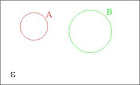
Axiom 3 is doing the work.  The idea of disjoint events is from set theory.  The following shows two disjoint events.

 And here's a pair of events which are not disjoint.

While this isn't the whole story on independence and mutual exclusivity, I won't go further on it at this point.

Axioms 1 and 2 allow you to synthesise some of the phenomena of relative frequencies without having to mention them - namely that, since a relative frequency is a ratio of one count over a second, larger, all encompassing count, it will always lie somewhere between 0 and 1.  Kolmogorov, after all, is re-modelling the foundations, not pulling down the entire edifice.

Axiom 3 is all about relationships.  This set of numbers, this probability distribution, clearly can't just be any set of numbers.  Some of those numbers relate to each other in a very specific way.  Axiom 3 states that there's a summation relationship (actually infinitely many of them) between a number and a bunch of other numbers precisely insofar as their referent events, which, remember are disjoint, when $\bigcup$-ed together equal each other.

Spelling it out for just one case.  Imagine there is an infinite set of disjoint events $e_i$.  Performed a set union on them all let's call the resulting set $E_i$.  $\forall e_i$ and the single $E_i$ both are already in your reference set.  Now that we have identified this set relationship between  $\forall e_i$ and the single $E_i$ we  make a corresponding claim about the set of numbers that constitute this particular probability distribution.  Let's call that set of numbers $n_1, n_2, ..., n_i$ and the single number $N_i$.  Axiom 3 tells us that we can be certain that $n_1 + n_2 + ... + n_i = N_i$

This isn't a moral point about gambling or even empiricism.  If anything it is motivated by an aesthetic-mathematical impulse.

At last, mathematical formulae on Blogger posts

See http://mnnttl.blogspot.com/2011/02/latex-on-blogger.html - it works for me.

Sucking the pips off

Around any randomisation machine humans build rules which allow you to throw away information.  How do you analyse this mathematically.  Here, somewhat artificially, I'll constrain the analysis to dice.

Imagine one die with no distinguishing marks.  What's the information content?  Yes, 0.  You learn nothing new on  each throw.  Mathematically, the information content is $-\sum{p_i \log_2(p_i)}$.  You can think of this as a single probability $p$  value $1$.

Now re-imagine the pips. This time $I = -6\times{\frac{1}{6} \log_2(\frac{1}{6})} = 2.6$ bits. You can still throw a pipped die and mentally decide to ignore the number which lands face up.  What have you done?  You've created in your head an equivalence class.  You've said to yourself, 'for my own purposes I will assume an outcome which is a combination of all six elementary outcomes'. Given each elementary outcome is independent, you can find the probability of your all-encompassing equivalence class as the sum of the elementary classes.  Let $E_c$ be your all-encompassing equivalence class  and $e_1$, be the elementary outcome of getting a 'one' face up, etc. Then $E_c = e_1 \cup e_2 \cup e_3 \cup e_4 \cup e_5 \cup e_6$ and, by one of the three basic axioms of probability, $P(E_c) = P(\bigcup_{i=1}^6 e_i) = \sum_{i=1}^6 P(e_i) = \frac{1}{6}\times 6$.

So, just by imagining it, you can turn off your randomisation machine.  The same trick can be used to turn your randomisation machine into a coin-flipper, which as you can guess, provides just $1$ bit of information.  Just imagine two elementary outcomes, even numbered pips and odd numbered pips.  So what you have is a randomisation machine which has a maximal amount of information on offer to you.  The rules of your game, your context, determine how you might want to throw some of that information away for the purposes of your game.  You've combined elementary outcomes.  So one die can deliver a uniform distribution of 6 events of probability $\frac{1}{6}$, or a coin flip.  You can see how you could imagine  randomisation machines giving two unbalanced equivalence classes, of probability $\left\{ \frac{1}{6} \frac{5}{6}\right \} I=0.65$ bits and  $\left\{ \frac{1}{3} \frac{2}{3}\right \} I = 0.9$ bits.  You could chose to implement this in a number of different ways.  For example, in the $\left\{ \frac{1}{6} \frac{5}{6}\right \} $ by imagining 'one pip' to be the first of your equivalence classes and 'either 2 or 3 or 4 or 5 or 6 pips' to be your second.  $E_1$ and $E_{2\cup3\cup4\cup5\cup6}$, if you will.  But just as good a job could be achieved by $E_2$ and $E_{1\cup3\cup4\cup5\cup6}$, etc.

Equivalence classes are a mathematically formal way of expressing the idea of treating one or more possibilities as coming to the same thing for your current purposes.  It maps out a geography of interest and that geography is only constrained by the granularity of the maximal information state of your randomisation machine (playing cards, for example, are more fine grained, since you can have $52$ distinct elementary outcomes).

  In the next post, I'll look at how to interpret multiple repeats of the die tossing experiment but I'll end by pointing out that, from an analytical point of view it doesn't matter if you consider multiple repeats as either happening simultaneously (you roll two  differently coloured dice) or serially (you roll the white die and note the result, then roll the blue die and note the result).  As long as you are consistent in which of the two parallel-roll dice you report first.  Since these two dice outcomes are genuinely independent, I'll show you how the informational additivity of independent random events works mathematically too.  This leads in to considerations about becoming indifferent to order or retaining order (combinations and permutations respectively).

This reminds me of the Samuel Beckett sucking stones extract from Molloy.

Tossing away information

Continuing from my initial analysis I would like to model the consequences of sheep bones (just like all other animals' bones) being white.

The crucial human animation in using sheep heel bones as random event generators is the act of tossing.  In the act of tossing, you loose knowledge of the order in which your four bones will lie.  This wouldn't be an issue if all four bones were of a different colour.  Or perhaps if the bones were marked not with 1,3,4,6 on each of the four bones, but with 16 different numbers.  If humans had etched 16 different numbers (pips) on their bones, they'd be using the maximum amount of information possible in that act, namely 6.88 bits.  But that doesn't happen.  Instead we humans make 4 more or less similar sets of markings on the bones.  Then, when we toss, we toss away some information.  But how much?

To answer this question, consider the die.  One die has 2.6 bits per roll.  With two dice, if order is important, then you have 5.16 bits (imagine each of the dice had a different colour).  With three, 7.75 bits (again, imagine each of the three dice a different colour).  You can see how when you run this experiment, information is additive as the sample space size grows multiplicatively.  You can also see that, with the addition of colour, your parallel toss does not lose track of which die had which value.  This parallel toss is the same as if you had tossed one die two (or three) times, and taken note of each result.  It is a kind of 'sampling with replacement' activity in so far as the probability of any single outcome is independent of earlier throws.  (The Markov property).

But bones are white.  And there's a pre-existing tradition of making each bone contain the same number and type of markings as each of the others.  Most likely early dice were crafted out of the astragalus, and they would have inherited this feature of being practically indistinguishable from each other.  That means, when two or three are tossed, information is lost, in comparison to the 'order important' experiment.  Of course, the lost information is precisely that of ordering.  But how much?  For two indistinguishable tossed dice you now only have 4.3 bits of information. When you do the 'order unimportant' analysis on four astragali, the information content drops from 6.88 to 4.3 bits.

Isn't that amazing?  Given what we know about the colour of bones, the number of sheep legs and the casual act of tossing collections of indistinguishable objects, we  built up a randomisation machine which would conveniently deliver for us 4.3 bits.  When we smooth and chip away at a sheep-load of astragalli and make them into 6 sided dice, we manufacture a convenient randomisation machine which delivers 4.3 bits of information to us using only two dice.  That is impressively close to the original.  All those religious-oracular rule books, all those long-forgotten games could still be randomised by a machine of approximately the same degree.  One die would not have been enough, three too much.  But two would have been just right.  Our culture got to keep the innovations built up around the astragali.

My guess as to why each bone (and, later, die) was marked identically is because in the beginning was the single astragalus.  It was a much easier step to make a second instance of that same pip-marked bone.  And a third, and a fourth.  

But why did humans go to the bother of crafting a die if their main practice of four-bone tossing is equivalently replaced with two dice tossing?  Was it a matter of aesthetics?  Did the cubic astragalus with only 4 landable sides present an affront to our sense of symmetry?  Surely it couldn't be to make any kind of mathematical analysis more amenable, though it isn't impossible that some people might have worked out the possibilities of dice.  My money's on our desire to manufacture a symmetric, crafted, more aesthetically pleasing randomiser machine.  The uniform distribution perhaps also made the construction of new equivalence classes and interpretive games based on that uniform element of randomness easier to plan and design.

Ground-hog Governor

I've been listening to the Bank of England quarterly inflation press conference for many years now, and it never fails to amuse just how many times Mervyn King can give in effect the same answer to everyone's various questions.  The fault lies not with Mr King, who I think does a decent job at these conferences, but the dolts in the press corps, who unfailingly ask the same badly-informed populist questions, again and again and again.  I have no idea why they do it, since they are by and large the same set of journalists who turn up each time.  Particularly at fault are the popular national newspaper economics journalists and their television colleagues (Sky, BBC, Channel 4, ITV) and the markets  journalists (Bloomberg, Reuters, Dow Jones).  The Economist journalists usually perform better.

They really ought to be ashamed of their performance.  Perhaps someone ought to edit out a chronological history, for each journalist, of the set of questions and King's responses directly to them, over the last 5 years.  Maybe then they'd get it.

Americans play craps because sheep walk on four legs

The sheep's astragalus can have its anatomically asymmetric shape scrubbed, chipped, smoothed so that it becomes a modern, more-or-less symmetrical, more or less fair die.  The first evidence for this happening, according to F.N. David is around 3000 B.C.  in Iran and India.  What does this allow?  Well, first, you now get a manufactured randomisation machine with an information content of 2.6 bits per die instead of 1.7 per bone.  This is achieved by there being six instead of 4 possible outcomes, in addition to the fact that they are now all, more or less, equally likely.

However, as David points out in her book, for thousands of years popular games and religious divination was performed with four bones.  You get a lot more combinations with four.  And the particular shape of the astragalus facilitates walking and running.  Bipeds, for example, would only have two such bones.  So for many millennia humans have been de-boning their sheep, four running astragali at a time, and inventing games and religious-oracular practices based on the resulting information revealed when the bones are thrown.  By my calculations, four bones rolled in parallel will result in a 6.88 bits of information being revealed.

Now, turning to the die.  If you roll one die, you get 2.6 bits of information.  Two dice deliver 5.16 bits of information, three, 7.75 bits of information.  If your culture had already invested several millennia worth of games of chance and religious divination based on the randomisation machine of choice delivering no more than 6.88 bits of information, you may not need the excess 0.87 bits of information implied in deciding to use three dice and may be content with the reduction in information implied in the pair of dice.

Take craps, for example, which is a slightly simplified version of the game Hazard.  These rules are a gambling cloak around a core randomisation/information generating  machine consisting of two tossed dice.  One of the steps in the game involves the active player making a choice between a target summed score of 5, 6, 7, 8 or 9.  There are close probabilities of winning associated with each of the five choices the player could make, but one had a clear edge - the choice of 7.  So clearly at one time, this knowledge was not widespread, and probably some regular players who worked it out would clear up at Hazard gatherings.  Eventually this kind of secret could not be kept private for too long.  Once everybody knows that you are best advised to pick 7 when faced with the choice, there's no real point in having that choice in your game rules.  The game rules morphed as a result in the 19th Century.  Why then?  Pascal, Fermat, Huygens were all long in their graves by then.   Perhaps it was as a result of the game-busting brilliance of Pierre Remond de Montmort, arguably the worlds first quant, insofar as he took a gambling practice and, through a clear-sighted analysis of the games, blew apart their inner logic and flaws.  One of his analyses was on the game of two dice Hazard.

He also worked on finding the sum of the first n terms in a finite difference calculation, which is of course a supremely quant-like activity.

Another way of looking at de Montmort's effect on Hazard is to say he made it more efficient.  By revealing seeming choices which, through analysis, were no choice at all, he invented the concept of a rational gambler.  And the effect of the rational gambler on games of chance was to put the weaker ones (both players and games played) out of business - or rather - to require them to become more efficient.  This is not so different from the way that the branch of relative value trading known as convertible arbitrage has had real effects on the terms and conditions of real convertible bond issues.

Knucklebone technology, degrees of certainty, Kolmogorov

Imagine that what we now commonly think of as the subject of probability is nothing other that three distinct areas of human intellectual effort, bound more or less uncomfortably together.

What's the best order to tell their story?  Historically, I suppose.

At some point in human pre-history, men became aware of degrees of certainty within their own heads concerning matters of the world.  This may or may not have happened before the invention of counting.  So these degrees were more likely to be rank-based.  I assume also that some people would have been substantially better at this kind of comparative ranking of possibilities than others.  I'm agnostic on whether they were on average any good (one of the findings of modern behavioural economics, for example, is just how bad we are at this kind of reasoning).  The exact dating of this period is most certainly lost to us.

Later mankind invented technologies which allowed them to create randomisation machines with more or less stable relative frequencies.  These machines are clearly out there in the world, as opposed to in people's heads.  As such, they provide the possibility for us humans to observe their behaviour when executed, to note the stability of their outcomes, and for these outcomes to be inter-subjectively affirmed.  Credit goes to part of the heel bones of deer and sheep - the astralagi - as the first randomisers.  These were approximately dice-shaped and were sturdy enough to be rolled on many primitive floors.  Because of their shape, when they landed, they did so uncontroversially (as opposed, for example, to a walnut, about which there could be much dispute, I'd imagine, over exactly which way up it landed, and as opposed to, for example, a toe bone, which would mostly land one side or the other and could probably be gamed easily).  Two of the six sides in this approximately die shaped object were rounded and hence when you throw it, won't land on those sides.  Of the remaining 4 sides, two were approximately likely to be seen 2/5 of the time, and the other two both about 1/10 of the time.

When you're playing games which contain an element of randomness, then if you chose a coin-like object, you have to execute its randomisation operation (toss it) more times to reach the same degree of randomness.  In object-scarce primitive times, it is probably practically more useful, not to say more fun, to use a randomiser with 1.7 bits of information revealed per toss than one with just 1 bit.  1.7 bits represents the information content  in a discrete probability distribution with values {2/5, 2/5, 1/10, 1/10}.

Such activities as rolling the astralagus presented a stable real world phenomenon (in the sense of delivering stable relative frequencies) against which one could measure up one's own subjective estimations of certainty. Notice that it is easy to imagine a world which had individuals making subjective cardinality comparisons between possible futures, in the absence of any randomisation machine; but not vice versa.

The beginnings of an analysis of the properties of these randomisation machines heralded the birth of the frequentist approach.  We've moved on from the astralagus to Chaitin's algorithmic complexity.

Finally we have Kolmogorov replicating the essential rules of the frequentist approach into the axioms of a brand new branch of logic or set theory - using measure theory to achieve that goal.  The frequentist analysis thus seems to be the crucial link between the uncertainty of subjective approaches and the formality of set and measure theoretic definitions of probability.  But while the set theoretic approach renders the common axioms of the frequentist approach well, it doesn't rely on frequentism to derive any of its conclusions.

Who do you love? Syntagmatic and paradigmatic dimensions of Homo Economicus

Who does economic man care about?  'Himself' is probably most people's first thought.  Rightly so.  But can we come up with a better answer?  Or perhaps it is an answer to the related question: who ought economic man care about?  Clearly this is a moral question.

What kinds of different answer could there be?  To answer this I'll make reference to two dimensions of analysis from the subject of semiotics as laid out by its originator Saussure, namely elaboration of the meaning of a sign along the syntagmatic and the paradigmatic dimensions.

When considering how widely or narrowly economic man could cast his net, we can fix the widest and narrowest point.  The narrowest point sees economic man making his calculations based on his current set of desires and feelings, with no consideration to the economic man he will become in the future.  This I'll call the minimal or instantaneous economic man.

The widest point has each and every economic agent consider all humans who ever lived, who are living, or who ever will live.  This is a quasi-spiritual position and would clearly be hard to implement, but implementation cost has never been the subject of concern for the founders of the model of economic man.  Compare some major world religions, for example, in the scope of their caring - Christianity seems to cover the moment, Shinto covers the moment and the past, Buddhism covers the moment and the future (it's even extended beyond humanity itself).  I'll call this model the congregation of economic brothers.  

It seems strange to step into what has formerly been the realm of religion and morality but I'm thinking of a cold hard piece of formal mathematics, and equation, which (somehow) has to try to capture this concern.  This piece of mathematics, this set of equations, could themselves be the inspiration of just as many fruitful directions of intellectual advancement as did the mathematical formalisation of the economic man of classical Ricardian economics (classical economic man).

Comte came closest to this in the recent humanist intellectual  tradition in his 'living for others' dictum, including all currently living humans, but excluding antecedents and descendants.  

If these are our intellectual boundaries in this search, how do we execute that search.  Saussure extended the linguistic observation of words (signs) having a meaning or relevance by virtue of where they are placed in the sentence (the syntagmatic dimension) and by virtue of which word (sign) was chosen for this sentence, compared to the other words which could have been chosen in that place (the paradigmatic dimension).

This partly relates to the social statics (paradigmatic) and dynamics (syntagmatic) perspectives  in economics generally.  Here, history or evolution is either held constant or not and the analytical consequences of that decision are investigated.

All it takes is for instantaneous economic man to become interested in his future self and we arrive pretty quickly at classical economic man.

It is in theory possible to consider a bizarre model of economic man where he doesn't consider his own utility but someone else's - perhaps randomly chosen.  I'll call this the economic surrogate. 

 If this surrogate relationship embodied a permanent fix to the other, then surely a world of economic surrogates would look like the world of classical economic man, except one where the surrogate/beneficiary could be considered to be classic economic man himself, with the additional detail that he outsourced the calculation to his 'slave'.  Again, the implementation of this scheme might be well-nigh impossible due to the unlikelihood of the decider  knowing much about the beneficiary's motivations or perhaps even preferences  If, on the other hand, the random association to the other beneficiary was itself becoming randomly attached from one to another beneficiary, then perhaps its macro-effect wouldn't be too different from a congregation of economic brothers.

There's a more natural sounding direction toward which our utility maximiser widens his scope of caring - towards the family.  (Or the household, to give it a more familiar ring).  Clearly many parts of economics are happy to consider meaningful aggregations of agent - households, firms and governments being three obvious aggregations.  I'll call economic man who cares about maximising the utility of his family the economic father.

Push this concern out beyond the set of descendants he's likely to meet to all of his descendants, and you're well on the way to the congregation of economic brothers again.  There's no point in considering predecessors since they don't make decisions and don't need a utility maximising machine.  However, households and families, while often being co-existent, don't always in the general case need to be - households can consist in many non-family members.  Let's accept that the economic father can have genetic and co-habitee elements.

You'll have noticed that, aside from the computational complexity of these 'maximising N utility functions' approaches, you also have the practical difficulty of really knowing the preferences of all other others.  This isn't fatal, I don't think, since there are reasonable philosophical arguments for questioning infallibly introspecting one's own preference set.

Just as soon as you start maximising N utility functions you begin to wonder if all N utility functions are equally important to you.  In more artificial permutations of economic man (surrogate, congregation) implicit is a thought that each time you get assigned to a surrogate, or if you're in the congregationalist model, the weightings are fair (in the mathematical sense).

But for the economic father it might be quite acceptable to weight closer relatives or co-habitees with higher fractions of your own brawn towards the goal of maximising their happiness.  If in the limit you weight your own utility with 1.0 and everyone else of the N-1 with 0, you're back to classical economic man.

An exponentially declining weighting could be imagined, whereby everyone in your utility-maximising team could be ranked and placed on that list.  That way you can apply discount factors to future possible generations.